Transcription
The Electrical Control and Energy Management System of aUniversity: University of Texas a Case StudyFrederick C. HuffEmerson Process ManagementPittsburgh, PARoberto Del Real, P.E.University of TexasAustin, TXSteve PayneEmerson Process ManagementPittsburgh, PA
SummaryWho;University of TexasWhere:Austin, TexasWhen:Site Visits: December, 2007;April, 2008What:Electrical Controls and Energy Management SystemsKEYWORDSElectrical Control, Energy Management, Load Shedding, Demand Control, Reactive Power ControlABSTRACTA university campus like many manufacturing processes require large quantities of process steam as wellas power for their operation and it is common for these energy sources to be provided by a captive powerplant, with any shortfall in generated power being drawn from a local utility tie-line. Electricaldisturbances such as interruption in service from the utility or tripping of a generator can cause overloadand instability problems and lead to the loss of process and power functions unless corrective action istaken immediately.In addition to process steam and real power demands, a campus can also have a varying reactive powerdemand that must be satisfied. Reactive power affects line currents and bus voltages, as well as powerfactor of the tie-line bringing power into the plant from the local utility. The local utility can apply apenalty if the tie-line power demand exceeds an agreed value, and can conceivable impose a low powerfactor penalty as well. Stable system operation requires that bus voltages are maintained within assignedlimits, that transformers and connecting cables do not become overloaded, and that generators run withintheir reactive capabilities.Hence the campus power house needs an electrical control and energy management system to providecomputer assisted control in the areas of: Tie-line or Demand ControlReactive power controlLoad SheddingThe University of Texas at Austin needed a state of the art electrical control and energy managementsystem for their power house. This paper discusses why the system was necessary and the objectives ofthe system. It then describes the DCS system configuration and functions that were provided.
The Electrical Control and Energy Management System of aUniversity: University of Texas a Case StudyIntroductionThe University of Texas at Austin (UT) is a major research university located in Austin, Texas and is theflagship institution of The University of Texas System. The university was founded in 1883 [1], and hashad the fifth largest single-campus enrollment in the nation as of fall 2007 (and had the largest enrollmentin the country from 1997–2003), with over 50,000 undergraduate and graduate students and more than16,500 faculty and staff. It currently holds the largest enrollment of all colleges in the state of Texas.The Main Campus Power Plant and Central Chilling Stations with a current capacity of 112 MW and40,000 Tons respectively provide electricity, steam, and chilled water to campus. In 2005 the Campusexperienced two unfortunate total black outs causing disturbances through out. During root causeanalysis sessions and action items discussions, it was noted improvements needed to be made in theelectrical control system to prevent further total power loss events.In addition to the noted needed improvements, the decision was made by University officials to get theGeneration Plant ready to sell power due to the always attractive big potential financial benefits involved.The Generation Plant had a control system in place at the time of the two outages which was not capableof responding to the need for load shed and tight demand control. Emerson Process Controls wassubsequently contacted and discussions began for the design and implementation of a load shed systemas well as to improve the demand load control system.UT Power SystemAn essential element in maintaining the success of the University of Texas as an education and researchinstitution is a state-of-the-art and highly reliable electric power system. To ensure reliability, powersources include utility steam power boilers, combustion and steam driven turbines. The distributionsystem which is the last section of the electrical power system is a loop connection designed withredundancy throughout the campus to provide a high level of service continuity and operating flexibility.The campus is served from the local utility with four 69Kv services as shown in Figure 1, with preparationto be served in the future with 135Kv already in place. Each of the four active utility services is thentransformed down to 12Kv and connected to the main switchgears. Both Combustion Turbo-generators(CTG’s) and two of the four Steam Turbo-generators (STG’s) produce power at 12Kv, the other twoSTG’s produce power at 4.16Kv which served a minimum number of older buildings in Campus. Themaximum amount of internal power available is approximately 112MW with short term plans to increaseto 127MW by the acquisition of a 35 MW CTG. Under the current contract the university can purchase25MW from the utility on an emergency basis.The distribution system load varies during the day. The maximum load occurs in the early evening or lateafternoon, and the minimum load occurs at night. The design of the distribution system requires thecontrol system to determine and manage voltage during high-low load conditions because the voltagedrop is at maximum during peak load and over voltage may occur during the minimum load. Voltagecontrol for generators and capacitor banks installed in key areas of the distribution system are keycomponent of the highly reliable system. The control of the distribution system is accomplished via astate-of-the-art SCADA (supervisory control and data acquisition) system running on a redundant serverenvironment and communicates with external instrumentation and control devices. Communicationmethods are via two fiber rings, Ethernet, and OPC (OLE for process control) links. The SCADA programhas a database which tells the software about the connected instrumentation and which parameterswithin the instruments are to be accessed. The database may also hold information on how often the
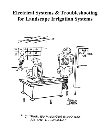
parameters of the instruments are accessed and if the parameter is a read-only-value or read/write,allowing the operator to change a value.Figure 1A one line diagram of the steam and power system is shown in Figure 2. There are four utility boilers andtwo Heat Recovery Steam Generators (HRSG’s) that produce steam that feed a 420PSIG header. Thetemperature of the steam in the header is approximately 725oF. Boilers 3 and 4 can burn fuel gas or oiland produce a maximum of 150Klb/H and 500Klb/H of steam respectively, they also have been retrofittedto meet tighter Texas environmental standards for low NOx. Boilers 1 and 2 are only used for emergencysituations when the main boilers are not available.The two CTGs are gas fired and the hot exhaust feeds the HRSG’s. The HRSG’s have supplemental fuelfiring by means of Duct burners. The throttle steam flows for the four STG’s come from the 420PSIGheader. All STGs have a condenser and three of the four have a 165PSIG extraction system. When aSTG is on there is a minimum amount of steam that must flow into the condenser.The acquisition of a new GE LM2500 25 MW combustion gas turbine paired out a new HRSG is on itsway and the goal of the University Utilities team is to have the unit operating by end of 2 010, this CTGwill replace the older 12 MW unit giving the Campus additional 15 MW generation.There are presently eight electric chillers providing 32,000 Tons 39 Deg F chilled water to Campus, theremaining cooling capacity is provided by four steam driven chillers three of which will be phased out in2008. A new Central Chilling Station is to be commissioned in early 2009; the new chillers manufacturedby Johnson Controls/York will be electrically driven with variable speed drives to control compressor load.This upgrade will give the Campus additional 9,000 Tons of cooling capacity. A new inlet air coil system
connected between the new Central Chilling Station and the main CTG will also improve the efficiency ofthe turbine providing additional generation capacity to campus.University of Texas Steam and PowerOILMSCFHGASMSCFHMSCFHxx.x MWxx.x MWMSCFHMSCFHMSCFHMSCFHMSCFHCTG 8CTG 10AUTODROOPHRSG 8MSCFHAUTODROOPUB1UB2UB7UB3HRSG 10xx.x KLB/HPRESSxx.x KLB/Hxx.x KLB/Hxx.x KLB/HTEMP 420# STEAMxx.x KLB/Hxx.x KLB/Hxx.x MWSTG 9xx.x KLB/HPRESS165# STEAMxx.x KLB/Hxx.x KLB/Hxx.x MWxx.x MWxx.x MWSTG 7STG 4AUTODROOPMANDROOPxx.x KLB/Hxx.x KLB/HSTG 5xx.x KLB/HTEMPPOWERTIExx.x MWELECTRIC CHILLERSFigure 2The University of Texas campus has various power sources including multiple utility services, CTG’s, andSTG’s. Currently, the university satisfies the campus power demand from internal generation. However,with the ups and downs in the price of natural gas it may become more cost effective to purchase powerrather than generate it; there is also an initiative to sell power provided financial benefits are present.Some combination of the multiple power sources is required to supply the total campus load. The loss ofany one of these sources may result in the campus load exceeding the capacity available. In the event ofa contingency it is necessary to determine if the campus load will exceed the capacity of the remainingpower source(s). If the load exceeds the available capacity it is necessary to shed non-essential loads inorder to prevent overload of the remaining sources. Load shedding must take place before any of theremaining sources trips due to under frequency.Since the decision on whether to generate power or buy power varies based on the cost of fuel for thesteam and power producers it is necessary to have a control system that can easily adapt and control theinternal generation accordingly while ensuring that the amount of power purchased in any 15 minutedemand period does not exceed the demand limit.In addition to process steam and real power demands, there is also a varying reactive power demand thatmust be satisfied. Reactive power affects line currents and bus voltages, as well as power factor of thetie-line bringing power into the plant from the local utility. Presently, the local utility applies a penalty if thetie-line power demand exceeds an agreed value, and it can decide in the future to impose a low powerfactor penalty as well.A stable system operation requires that bus voltages are maintained within assigned limits, thattransformers and connecting cables do not become overloaded, and that generators run within their
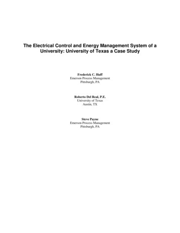
reactive capability curves. Therefore, there is a need for an Energy Control and Energy ManagementSystem (ECEMS) to control and manage the devices that affect the internal active and reactive powergeneration.The ECEMS installed at the University of Texas contains the following primary functions:1.2.3.4.Tie-line power monitoring.Demand ControlHigh speed contingency analysis and load shedding.Reactive Power ControlSystem ConfigurationAt the UT campus the breakers that had to be automatically shed are located at different switchgear andstations and buildings all around campus. In order to shed the breakers in a fraction of a second all of thetrip commands and the open and closed indicators had to be hardwired into the system via remote I/Oracks connected through a fiber link to the main load shed controller. All the automatic shedding breakersand the breakers that had to be checked to see if a contingency occurred (i.e. loss of grid) werehardwired via remote I/O into one redundant controller. The logic in this controller runs at 50 msec. Figure3 shows the basic structure of the Distributed Control System (DCS). The analog data such as amps,volts, MW and MVAr come into the system over a redundant OPC link from an existing SCADA systemwhere the operators also manually operate the breakers.SCADA SystemOPC LINKMMIENGREDUNDANT PCLoad Shed LogicHSRDataHighwayCONTROLLERHigh SpeedLoad Shed Controller50 msecCONTROLLERDemand ControlReactive PowerControlRemote I/O to Load Shed BreakersFigure 3Another redundant controller was provided to perform all the demand control and reactive power controllogic as well as issue commands to the generators. A redundant PC was supplied for the OPC link to theexisting SCADA system and to the Plant auxiliaries PLC system plus it also contained high level loadshed logic.
The data scanned at each location is made available at the main control room and all other controllers viaa redundant data highway. Time critical data is broadcast an updated in the memory of all drops every100msec. All non-critical or data used in control logic that can execute once per second is updated everyone second. This data is also available for viewing on operator stations. The data values are updatedonce per second on the operator station diagrams. The digital and analog values required in the loadshed system are scanned every loop time. This logic runs in a 50 msec loop. From the operator stationsin the control room the operators are not only able to monitor, but they are also able to perform controlactions such as changing of set points, on-line tuning of controllers, and the changing of controller modes(Auto to Manual etc.) The system also has the ability to store historical data that can be used not only inshift and daily reports, but also can be displayed in trend form that aid in analyzing the plant operation. Allof the DCS highway data is updated once per second at each operator console. The PCs based operatorconsoles are also able to originate highway points. Therefore, the results of a custom application programrunning in a PC can be made available to all other drops in the system as process point data.Tie-Line Power MonitoringUnder normal conditions the internal generation of the campus is sufficient to satisfy the electricaldemands with zero or a very small amount of power being purchased. However, if a generator is out ofservice purchased electrical power will increase. Also, in the future, conditions may change where theuniversity may decide to purchase power. Therefore, it is important to monitor the amount of purchasedpower over every demand period and ensure that the average MW consumption does not exceed thedemand limit defined in the utility contract. As stated in [2], demand is defined as the number of kilowatthours of electrical energy consumed during a period divided by the length of the contractual time window.At UT the demand period is 15 minutes. When the plant is connected to the Tie Line, demand limit error iscalculated as a prediction of the error that would be experienced at the end of the present 15-minutedemand period, if nothing were to be changed. Figure 4 shows the geometry of the demand periodcalculation in which is known: The time into the present period.The integrated energy consumed during the period expressed as MWH/H MW.The present Tie Line power in MW (ie) the slope of the line to the right of point t.From this information, the predicted error at the end of the period can be computed. In order to minimizethe frequency, with which turbogenerator adjustments are made, upper and lower deadbands are appliedto the calculated error. The magnitude of the deadbands are made to decline at the end of the period, andeven eliminated if the error was high at the time.Since UT does not receive a pulse from the utility company indicating the end of a 15-minute demandperiod, a "Sliding Window" control scheme is implemented. Three 15-minute windows that are phased 5minutes apart, execute every second and the largest calculated predicted error of the three windows isused for control. When this error is positive an alarm is generated so operations can decide if load shouldbe shed.
Load usage (MW h)Tie-line geometry} Demand errorDemand limit (MW h)Present usage (MW h)tTime (minutes)15Figure 4Demand ControlThe primary goal of the generator load control logic is to perform demand control. The function of thislogic is to control the loads on the available STGs and CTGs such that the amount of power that ispurchased from the utility is equal to the desired amount of purchased power entered by the operator.This logic is also used to provide a cost savings when the plant is connected to the grid. If it is cheaper tobuy power rather than generate power, then the operator should enter a set-point for desired purchasedpower equal to a value very close to the demand limit defined in his utility contract. If it is cheaper togenerate power rather than buy power, then the operator should enter a very low set-point, say .1 MW. Ifthe University wishes to sell power to the utility grid, then the operator should enter a negative set-point.As described in [3] combined cycle operation is where the exhaust gases from the gas turbine are used toprovide the heat necessary to produce steam that is fed into a steam turbine making the efficiency higher.Inside the UT power house steam can be made from HRSG’s and/or gas fired boilers. Clearly it is mostefficient to supply steam from the HRSG’s rather than the boilers. Therefore the following steps outlinethe sequence in which the loads are controlled on the STGs and CTGs when all of the generators areconnected to the grid: Allow the CTGs to reach their maximum MW load while keeping a minimum MW amount onthe STGs based on current process steam demand and minimum condenser flow. Once the CTGs are at maximum load, the STGs will increase in load until their maximum isreached or the available amount of 420 psig steam is exhausted. If the plant’s internal generation is at its maximum, and the plants power demand continuesto rise, the amount of power purchased from the utility will increase. If the plants internal power demand continues to rise such that the amount of purchasedpower will exceed the demand limit, automatic load shedding can occur or the operator candecide if loads should be shed.Some of the generators are controlled by issuing raise/lower pulses and others require a 4-20ma analogsignal.
Contingency Analysis/Load SheddingAccording to New [4] any part of a power system will begin to deteriorate if there is an excess of load overavailable generation. The prime movers and their associated generators begin to slow down as theyattempt to carry the excess load. The sudden loss of generating capacity on a system will beaccompanied by a decrease in system frequency. The frequency will not suddenly deviate a fixed amountfrom normal but rather will decay at some rate [5].The initial rate of frequency decay will depend solely onthe amount of overload and on the inertia of the system. However, as the system frequency decreases,the torque of the remaining system generation will tend to increase, the load torque will tend to decrease,and the overall effect will be a reduction in the rate of frequency decay. Assuming no governor action, thedamping effect produced by changes in generator load torque will eventually cause the system frequencyto settle out at some value below normal. If governor action is considered, and if the remaining generatorshave some pickup capability, the rate of frequency decay will be reduced further and the frequency willsettle out at some higher value. In either case the system would be left at some reduced frequency thatmay cause a further decrease in generating capacity before any remedial action could be taken.Excess load is usually caused by an electrical disturbance such as loss of tie-line power or tripping of agenerator. Traditional ways to minimize the effects of these interruptions usually centers on conventionalunder-frequency load shedding. The loads to be shed are often grouped by priority [6]. Loads assigned tolevel 1 can be disconnected first. Loads pertaining to level 2 up to the maximum level can bedisconnected in sequence of importance. The frequency of the plant is monitored and loads are shedaccording to the drop in frequency. For example, 59.85 Hz corresponds to no shed, 59 Hz mightcorrespond to level 2 shed, 58 Hz corresponds to level 3 etc. Load shed systems based strictly on underfrequency generally do not provide the operator with the ability to modify the set of breakers that areavailable for load shedding. The breaker set is fixed. In addition, in these types of systems the amount ofload shed is fixed and usually greater than the actual amount required.System modeling work has been done to allow the electrical engineer to simulate actual disturbances andexamine dynamic responses [7,8]. In order to do this the models must contain the inherent gains and timedelays in each components transfer function [8]. The purpose of the modeling is to identify the amount ofload that must be shed for a drop in frequency caused by a contingency. This is a difficult task andrequires accurate models for the load amounts to be accurate.Alternatively, the amount of power being produced can be constantly compared to the amount of powerbeing consumed to make sure they balance. The load-shed system can continuously monitor the state ofthe plant electrical system for “contingencies”. These are unplanned trips of power producers that wouldlead to a power imbalance. If the amount of power lost by the tripping of a power producer can be madeup quickly by the power producers connected to it no load has to be shed. However, if the spare capacityof the remaining power producers is insufficient to make up the load lost by the trip, then load must beshed. For example, if a plant generator trips and there is also a utility tie-line connection on that portion ofthe plant, the amount of power lost from the generator will automatically be supplied by an increase ofpower through the tie-line. This type of load shed system was installed at the University of Texas.The UT electric power system has four tie-line connections but all four must be lost before the tie-line islost, two Combustion Turbo-generators (CTG), and four Steam Turbo-generator (STG), making a total ofseven power producer contingency cases. The load shed system constantly monitors the amount ofpower being produced by each one and the spare capacity of the power producers connected to eachone. If one of the power producers is lost the amount of load that must be shed is equal to the amount ofpower lost minus the spare capacity of the power producers connected to it.When the plant is connected to the grid the base frequency of the plant is set by the grid power. In thisconfiguration the in plant generators run in droop mode. However, when the entire plant, or a portion ofthe plant, becomes an island, frequency must be maintained. Therefore one of the in plant generatorsmust be placed into isochronous mode while the others remain in droop. When the plant is disconnectedfrom the grid the frequency of the generator buses must be monitored. If the frequency of the bus starts todecline load must be shed before the bus frequency reaches a level that will cause the generatorconnected to it to trip. UT has six generator buses thus there are also 6 bus frequency contingency cases
in the load shed system. The frequency of each generator bus is hardwired into the DCS so the busfrequency can be monitored every 50msec.This load shed system consists of a program that runs every three seconds in a redundant Windows PCthat constantly performs a "What-If" analysis. This program does not check for the loss of a powerproducer, but rather it constantly calculates the amount of power that has to be shed if any of the powerproducers are lost. Then for each possible contingency case the program marks breakers to be shed incase this contingency case should occur. The breaker selection is based on breaker availability, locationof the breaker (was it powered by the power producer), and its priority. The University electrical teamhardwired a total of 65 contingency breakers throughout Campus for load shedding purposes; all of thesebreakers were individually functionally tested during project commissioning. All generators breakers werealso hardwired to the remote I/O rack connected via a fiber link to the fast speed controller. The prioritiesof the breakers are set by the operator and can be changed at any time. Every time this program runs itexamines the current status of all of the plant breakers and their values and determines which bus eachbreaker is currently powered from.In the DCS controller logic runs every 50msec that checks all the breaker statuses. Whenever, this logicdetermines that a contingency has occurred it automatically issues the trip commands for those breakersthat were ARMED for this contingency case by the load shed program that runs in the redundant PC. Theresponse time of the fast load shed redundant controller was tested during commissioning by simulating atrip of a generator and the actual shedding of a chiller; the total system response time from generatorbreaker open to chiller open signal status acknowledgement was recorded at 80 msec.Whenever loss of tie line is detected in the controller a command is sent from the DCS to one of the inplant generators to automatically switch the mode of the machine from droop to isochronous mode.The operator uses the graphic shown in Figure 5 to change the priority of the breaker and to inhibit it frombeing shed. A breaker with a low priority is shed before one with a higher priority. This screen alsoprovides the operator with the ability to enter a default MW amount for a load shed breaker. The open andclosed indicators are hardwired but the MW values come over the OPC link. If the indicators prove thatthe breaker is closed and there is a load the default MW amount is used by the load shed system whenthe MW value coming over the link is bad or if there is a problem with the OPC link.
Figure 5Diagrams as shown in Figure 6 exist that informs the operator which loads will shed if a contingency caseshould occur. The MW value of each breaker that is ARMed appears in the proper contingency casecolumn. At the top of the diagrams the amount of power being produced is displayed along with the totalamount of armed loads. If the operator sees that a load will shed and he does not want it to, he can inhibitthe load or raise its priority.For frequency drop cases, the table shows the current frequency, and the amount of armed loads.
Figure 6Reactive Power ControlIn addition to the real power consumed by electric motors, lighting and other power consumers there is avarying reactive component which affects line currents and bus voltages, as well as the power factor ofthe tie-line bringing power into the campus from the local utility. In addition to applying a penalty if tie-linepower demand exceeds an agreed value, the utility often imposes a low power factor penalty as well.Meanwhile, stable system operation requires that bus voltages are maintained within assigned limits, thattransformers and connecting cables do not become overloaded and that generators and synchronousmotors run within their reactive capabilities.The objective of the reactive power control logic is to satisfy the University’s reactive power demandswithin the following operating constraints: Minimize the VAr flow in the networkKeep the generators within their reactive capabilitiesThis will lead to the following benefits: Reduce the VArs imported from the utility grid, thus improving the purchased power factor
Drops or rises in reactive power requirements of loads on a generation bus leads to fluctuations in thevoltages on the generation buses. If the VArs generated by the generators on that bus are adjusted, sothat all bus VAr demand is satisfied, the voltage on the bus will improve.The control strategy implemented at UT was to try to satisfy the reactive demand on a bus by the devicesconnected to it thus eliminating or reducing the flow of reactive power in the system. The first line ofdefense is the capacitor banks. When the reactive demand on a bus exceeds the amount of MVArproduced by the capacitor bank it should be turned on.On each generator bus that generator tries to make enough reactive power to satisfy the reactive demandon the bus plus any reactive power flowing into to it. Thus capacitors try to balance the load VAr demandon a capacitor bus at its local level, while generators try to minimize the VAr flow in the network from ageneration bus. Any further excess VAr demands are met from the utility grid.Optimizing both the load VArs and the VAr flows automatically optimizes the VArs imported from the grid.In order to ensure generators do not become overloaded the reactive capability curves of the generatorsare modeled in the control system. The estimated reactive capability curve for a typical generator isshown in Figure 7. As discussed in [9] the active power (MW) is plotted as abscissa and reactive power(MVAr) as ordinate. All the curves are arcs of circles. In general the reactive capability curve for agenerator can be divided as either over-excited (lagging) or under-excited (leading), depending onwhether the VArs produced is positive or negative.An important concept in the reactive capability curve is the power factor, which is defined asPF ww2 v 2,where w is the active power and v is the reactive power.The lagging portion of the curve can be divided into two parts where each part is a segment of a circle.When the rated power factor is 0.85 the arc starting about the origin and typically labeled between 1.0 to0.85 power factor (region I) represents the limit imposed by the condition of constant armature currentwhereas the other arc (typically 0.85 to 0 power factor in region II) by constant field current. The leadingportion of the curve can also be divided into two parts. The portion from -0.95 to 1.0 (in region I)represents the limit imposed by constant armature current and is an extension of the arc from powerfactor 1.0 to 0.85. T
plant, with any shortfall in generated power being drawn from a local utility tie-line. Electrical disturbances such as interruption in service from the utility or tripping of a generator can cause overload and instability problems and lead to the loss of process and power