Transcription
NEUBrewNOAA-EPA Brewer NetworkStrayLightCorrection.pdfFile NameStray Light CorrectionIntroductionScattering by the grating is the dominant source of stray light in grating spectrometerslike the Brewer MKIV. However, holographic gratings have lower stay light for higherline density. Therefore gratings of the following three Brewer models have stray light inthe following descending order: MKIV, MKII, MKIII. Other sources of stray lightinclude: (2) scattering by mirror surfaces, (3) scattering by surfaces of lenses and filters,(4) scattering by striae and inclusions in optical materials of lenses and filters, (5)multiple reflections between surfaces of lenses and filters that create weak out of focussecondary images, (6) Rayleigh and Mie scattering by air and dust particles in the airwithin the spectrometer, (7) scattering by housing surfaces, (8) Rayleigh scattering by thevolume of glass and fused silica, (9) distortions due to thermal gradients in the air withinthe spectrometer, and (10) diffraction on the apertures. There are also ghosts caused bygrating defects. Both the grating ghosts and specular reflections (glints) from apertureedges and optical element mounts are strongly wavelength dependent.Due to instrument contamination with dust the stray light is expected to increase afterfield deployment. This may have a larger relative effect with the MKIII (in the secondspectrometer of the double) with a grating that scatters less than in the MKIV with alower groove density grating that scatters more.The stray light results in a finite out-of-band rejection (OBR), meaning that light of othermore distant wavelengths than those specified by slit function’s fwhm also contributes tothe signal. The finite OBR causes significant error or spectrum distortions in regionswhere strong absorption or emission bands occur. In UV solar spectrometry the HartleyHuggins ozone band precipice (280nm-310nm) is particularly affected by thespectroradiometer’s OBR.If stray light is not corrected in UV scans, the calculated UV index is too large. Also, indirect sun observations (DS routine) stray light results in underestimated ozone columnfor larger air masses. In this document we concentrate on stray light correction in UVscans that we employed in generating 201 and higher UV scan data levels. This methodmay lead to a similar stray light correction of DS data. However, it was not tested priorto preparation of this document.We show results both from simulations and statistical summary from stray lightcorrections of actual data from eight network Brewers.Spectrometer integral equationMathematically speaking - it can be shown – that a spectrometer acts as a linear integraloperatorCreated on 6/5/08Prepared by: P. Kiedron, P. Disterhoft and K. LantzPage 1 of 26
NEUBrewNOAA-EPA Brewer NetworkStrayLightCorrection.pdfFile NameC(p) I( )r( )S(p, )d (1)that maps a quasi-monochromatic (fwhm 0) irradiance I( ) onto the electrical signal (orcounts) C(p), where: (1) p is the grating position and it is expressed in units ofwavelength, (2) r( ) is the quasi-monochromatic responsivity, and (3) S(p, ) is the filterfunction as a function of and the slit scattering function as a function of p. The filterfunctions are normalized: S(p, )d 1 for every p(2)In detector array spectrograph based spectroradiometer a snapshot of a spectrum for allwavelengths is taken simultaneously. Then eq. (1) in principle can be solved with respectto I( ) or in other words, a perfect stray light correction is possible. The stray lightcorrection via the solution of eq. (1) was described and used for detector array basedspectroradiometer (RSS) in Kiedron et al. (2002). See also Seim and Prydz (1972),Brown et al. (2003) and Zong et al. (2006) for matrix based methods.Note 1: The stray light effect is zero if I( )r( ) const. Consequently, by selecting a responsivity thatproduces smaller variance in r( )I( ) reduces the stray light effect. In UV-RSS the stray light is reducedby using dynamic range compressing fore-optics (Kiedron et al. 2001) and in VIS-RSS two color glassfilters are used for the same purpose. (Kiedron et al. 2002). The dynamic range reduction approach isachieved at the cost of lowering the signal-to-noise ratio.In a scanning spectroradiometer like the Brewer irradiance changes during a scan. Foreach grating position p the irradiance I( ) Ip( ) as the sky is different at differentinstances of p ( the position p is a linear function of time). Thus, instead of one equationwe must write a set of N equations:C(p) Ip( )r( )S(p, )d , p 1, ,N(3)In the general case this set of equations cannot be solved with respect to N vectorsIp1( ) , IpN( ) (each is N long) with only N measurement values C(p1), ,C(pN). In thecase of clear and stable sky Ip( ) vectors are not independent and they change with p in aregular way via sun zenith angle (SZA). Then an exact stray light correction is possible,however, it is achieved through a rather cumbersome process of irradiance extrapolationand synthesis.Stray light in the UV scan is a dominant component of the signal C(p) at the shortestwavelengths. Thus the level of stray light can be estimated directly in each UV scan andits value is C(p) at p for which the irradiance is practically zero. Accuratecharacterization of an instrument, i.e. knowledge or r( ) and S(p, ) functions is then notneeded. The value of the stray light can be subtracted from the signal. This amounts to apartial stray light correction. The efficacy of this approach is evaluated with simulationsin the next section. We also analyze the role of stray light in ozone retrieval.Created on 6/5/08Prepared by: P. Kiedron, P. Disterhoft and K. LantzPage 2 of 26
NEUBrewStrayLightCorrection.pdfNOAA-EPA Brewer NetworkFile NameSimulations of stray light and its correctionWe use eq. (1) to perform stray light simulations and estimate the quality of stray lightcorrection. To perform simulations we must estimate the quasi-monochromaticresponsivity and filter functions.In Figure 1 filter functions S(p,325nm) obtained with a HeCd laser for two MKIVBrewers are depicted. The difference between BR101 and BR114 as seen in Figure 1was confirmed with other measurements implying that a 0.5 order of magnitudedifference in the slit scattering function exists between seemingly identical Brewers.Note 2: It should be noted that the 1200 lines/mm holographic grating in the MKIV produces higher straylight than higher line density gratings of the MKII and MKIII Brewers. A ruled grating of the same linedensity would be expected to still have an order of magnitude larger stray light.For simulations we use the two slit scattering functions from Figure 1. We assume thatfor other than 325nm wavelengths slit scattering functions have the same wings. Thecentral part of the function however is replaced with triangular functions of fwhm thatchanges according to the anamorphic magnification of the Brewer spectrometer.Figure 1. Slit scattering functions for two Brewers measured during 1997 Intercomparison of UltravioletMonitoring Spectroradiometers (Lantz et al. 2002) (data from: ftp://ftp.srrb.noaa.gov/pub/data/CUCF/ ).The fwhm as a function of wavelength (green trace in Figure 2) is an approximation. Infact the fwhm most likely has a discontinuity at 325nm where the slit is changed duringCreated on 6/5/08Prepared by: P. Kiedron, P. Disterhoft and K. LantzPage 3 of 26
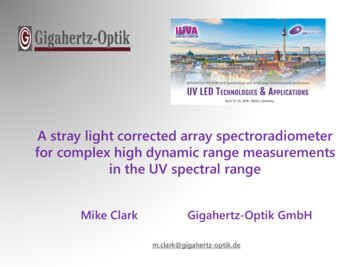
NEUBrewNOAA-EPA Brewer NetworkStrayLightCorrection.pdfFile Namethe UV scan. However exact values of the fwhm have a rather negligible impact on straylight simulations.Note 3: Many of the fwhm values for Hg, Cd and Zn spectral lines in Figure 2 are significant outliers. Thisis because some lines are not singlets and because of errors due to the inadequate sampling density. Thedata points for Figure 2 were taken from the 1997 Intercomparison of Ultraviolet MonitoringSpectroradiometers (ftp://ftp.srrb.noaa.gov/pub/data/CUCF/ ) without additional screening.Figure 2. Brewer MKIV approximate resolution (fwhm) as a function of wavelength (green trace).To reduce the effects of stray light the Brewer MKIV employs a solar blind filter (SBF)made of nickel sulphate hexahydrate (NiSO4.6H2O) crystal sandwiched between two UVcolored glass like Schott’s UG5 or UG11 (we do not know the exact glass used). TheSBF blocks longer wavelengths from entering the PMT’s cathode. The SBF is employedduring the UV scan for 325nm and during DS measurements.Note 4: The nickel sulphate based SBF has two leaks: 1% at 465nm and 6% at 895nm. The latter shouldnot cause problems as the cathode of the PMT used by the Brewer seems to have zero quantum efficiencyin the near IR. The 465nm leak, however may contribute to stray light during measurements. A separatetest would have to be performed to verify it. In our simulations we ignore this leak by setting r( ) 0for 363nm.In Figure 3 responsivities for p 325nm obtained using a lamp of known irradianceIlamp( ) are depicted. These responsivities are obtained from measured countsClamp(p) Ilamp( )r( )S(p, )d Created on 6/5/08Prepared by: P. Kiedron, P. Disterhoft and K. Lantz(4)Page 4 of 26
NEUBrewNOAA-EPA Brewer NetworkStrayLightCorrection.pdfFile Nameas followsRlamp(p) Clamp(p)/Ilamp(p)(5)For simulations we estimated the responsivity beyond 325nm based on SBF’stransmittance.Figure 3. Normalized responsivity measured with CUCF lamps in 286.5nm-325nm range and extrapolatedresponsivity in 325nm-363nm range based on the transmittance of the NiSO4 filter.Note 5: The responsivity of Brewer 154 (red) is expected to lead to higher stray light effect than theresponisvity of Brewer 139 (violet).Stray light in responsivityThe lamp based responsivity eq.(5) is affected by stray light. To obtain a quasimonochromatic responsivity r(p) one would have to solve eq.(4) or in other wordsremove the stray light from Clamp(p) counts before applying eq.(5). The solution of eq.(1)for static irradiance (like lamp irradiance) was described and used for array basedspectroradiometers (RSS) in Kiedron et al. (2002).Created on 6/5/08Prepared by: P. Kiedron, P. Disterhoft and K. LantzPage 5 of 26
NEUBrewNOAA-EPA Brewer NetworkStrayLightCorrection.pdfFile NameFor simplicity sake of our simulations instead of inverting the integral eq.(4) we setr(p) Rlamp(p) (where Rlamp(p) are from Figure 3) and then obtain the new Rlamp(p) usingeqs. (4) and (5). The lamp irradiance Ilamp( ) of a typical CUCF lamp (see Figure 4) wasused in eq.(4) to obtain the new Rlamp(p).Figure 4. Typical irradiance of CUCF FEL lamp.In Figure 5 we show the ratio of two responsivities: RC W(p)/RC(p), where RC(p) wascalculated assuming filter functions that have only central (C subscript) parts non-zero astriangular functions with a fwhm according to Figure 2. And RC W(p) was calculatedusing filter functions with the same central part C and with wings W from slit scatteringfunctions in Figure 1 for the two cases A and B. Calculations were done for allresponsivities from Figure 4 were considered as quasi-monochromatic responsivities ineq. (4). As expected (see Note 5) Brewer 154 has the largest stray light effect andBrewer 139 has one of the lowest. A less intuitive result is that a responsivity with straylight is lower than a responsivity without stray light in the region where a quasimonochromatic responsivity is maximum. One possible explanation for this is that thefilter function dissipates energy into its wings, which results in a reduced value of thesignal C(p) where r( )I( ) has its maximum (p ) in eq. (4).Created on 6/5/08Prepared by: P. Kiedron, P. Disterhoft and K. LantzPage 6 of 26
NEUBrewNOAA-EPA Brewer NetworkStrayLightCorrection.pdfFile NameFigure 5. Ratio of the responsivity with stray light to the responsivity without stray light for eight differentquasi-monochromatic responsivities and two slit scattering functions.The results in Figure 5 indicate that without an accurate characterization of an instrumentthat would allow correction of stray light, stray light in the responsivity alone may causesystematic errors of 0.3% in the 295nm-325nm region.Stray light effect in ozone retrievalDuring the DS measurement routine the direct sun irradiance is measured at fivewavelengths via five separate slits (i 2,.,6) at one grating position:Table 1. Brewer nominal slit valuesi ifwhm0303.21darkn/a2306.3 0.63310.1 0.64313.5 0.65316.8 0.66320.1 0.6From eq.(1) we calculate irradiance signals C( i) using as input N 1000 irradiancesI( ) I0( )exp[-x( )DUmo3 – r( )mr –a( )ma](6)where:I0( )x( )DUr( )– is the extraterrestrial irradiance (Bernhard et al. 2004)– is the Bass-Paur ozone cross-section at 229K– ozone column: random uniform in [150DU-450DU]– Rayleigh optical depth: random pressures P in [850mb-1050mb]Created on 6/5/08Prepared by: P. Kiedron, P. Disterhoft and K. LantzPage 7 of 26
NEUBrewNOAA-EPA Brewer NetworkStrayLightCorrection.pdfFile Namer( [µm]) 0.008569 -4(1 0.0113 -2 0.00013 -4) .(P/1013)a( )E(7)– aerosol optical depth is linear with wavelength:a(286.5) random in [0.01OD-1.01OD]a(365.0) k .a(286.5), where is k random uniform in [0.5-1.0]– solar elevation angle: random uniform in [0 , 88 ]and the air masses are calculated from the following standard equations:mo3– ozone air mass for h 22km, R 6370kmmo3 (1 h/R)/(sin2(E) 2h/R)0.5mr– Rayleigh air massmr (sin(E) 0.50572(6.07995 E )-1.6364)-1ma(8a)(8b)– aerosol air massma (sin(E) 0.0548(2.650 E )-1.452)-1(8c)Figure 6. Ratio of the signal with stray light to the signal without stray light for BR154 at six wavelengths(slit scattering function B).Created on 6/5/08Prepared by: P. Kiedron, P. Disterhoft and K. LantzPage 8 of 26
NEUBrewNOAA-EPA Brewer NetworkStrayLightCorrection.pdfFile NameIn Figure 6 the ratios CC W( i)/ CC( i) show the magnitude of stray light for sixwavelengths from Table 1.Ozone absorption is a chief cause of stray light effect. The smallest air masses lay alongthe lower envelopes of the scattered points in Figure 6. The points that lay about thesecurves are for cases of lower ozone values but large air masses. For large air massesRayleigh extinction becomes a significant contributor to the stray light effect.The four longest wavelengths are used to retrieve ozone. According to the Breweralgorithm irradiance signals C( i) for i 3, ,6 are used. The following quantities arecalculated for the four wavelengths:Fi log10C( i) r( i)mr(9)To replicate pressure uncertainty, as the Brewer uses only a nominal pressure for a givensite, we have added a 5mb pressure uncertainty when calculating r( i) for eq. (9).Ozone column DU is calculated from a linear equation:DUmo3 XSC(X - ETC)(10)whereXSCETCmo3- is the ozone cross-section constant (calculated)- is the extraterrestrial constant (measured)- is the ozone air massand X is a linear combination of measured signal irradiances:X a1 .(F5-F3) a2 .(F5-F4) a3 .(F6-F5)(11)where the coefficients a1 1, a2 -0.5 and a3 -1.7 are suppose (see Brewer manual) tomake the retrieval independent of extinctions that are linear with wavelength (chieflyaerosols).Note 6: Both coefficients XSC and ETC could be obtained using the correlation technique from anotherBrewer that is collocated and calibrated. This would be a transfer of calibration. In such a case the Brewerunder calibration becomes a secondary instrument. When XSC is calculated from characterization data ofthe Brewer, and the ETC is obtained from Langley regressions (DU is unknown but must be constant ineq.(10) in the Langley plot), then the Brewer under calibration will measure ozone from the first principles.We think it is very important to make a distinction between secondary and first principles instruments.XSC can be calculated explicitly using ozone x-sections and values of wavelength i.XSC can also be obtained implicitly from simulations like we have done here (see Figure7). In Figure 7 two simulated Langley plots are depicted. The coefficients XSC and ETCare obtained by fitting all of the points with an ozone slant path column DU.mo3 less thanCreated on 6/5/08Prepared by: P. Kiedron, P. Disterhoft and K. LantzPage 9 of 26
NEUBrewNOAA-EPA Brewer NetworkStrayLightCorrection.pdfFile Name1100DU. One can see that stray light affects XSC. XSC and ETC are different for the twocases.Figure 7. Ozone Langley plots to determine XSC and ETC coefficients.Figure 8. Ozone column retrieval errors in four cases. AOD is wavelength independent.Created on 6/5/08Prepared by: P. Kiedron, P. Disterhoft and K. LantzPage 10 of 26
NEUBrewStrayLightCorrection.pdfNOAA-EPA Brewer NetworkFile NameIn Figures 8 we show ozone retrieval errors, i.e., difference between ozone DUBrewerobtained from eq.(10) and ozone DU used in eq.(6) to calculate X with eq.(11). In thiscase aerosols are assumed to be wavelength independent. Four possibilities are shown:(red) retrievals when the data had no stray light; (green) XSC and ETC parameters usedfrom red case for data with stray light; (light blue) only XSC from the red case was usedand the ETC was adjusted using data with stray light; and (blue) both XSC and ETC weredetermined from data with stray light.We can conclude that XSC does not need to be determined using stray light data in thecalculations (light blue); however a small improvement is gained if it is (blue). The straylight significantly reduces retrieved ozone column. At 1500DU slant path ozone columna -26DU error is expected. Furthermore, we are somewhat surprised that in the no straylight case there is also a dependence on ozone slant path column (red).In Figure 9 wavelength dependent aerosol optical depths was added in simulations.Figure 9. Ozone column retrieval errors in four cases. AOD is linear with wavelength.On p.113 of the Brewer manual it is stated that “weightings [a2 -0.5 and a3 -1.7 ineq.(11)] remove the effects of absorption which are linear with wavelength”. Figure 9clearly does not concur. Perhaps because in our simulations we did not have exactly thesame filter functions ( i and fwhmi) as used by the Brewer and that we could have had anadditional wavelength shift error in the Bass-Paur spectrum with respect to what theBrewer is suppose to use.Created on 6/5/08Prepared by: P. Kiedron, P. Disterhoft and K. LantzPage 11 of 26
NEUBrewNOAA-EPA Brewer NetworkStrayLightCorrection.pdfFile NameFigure 10. Ozone column retrieval errors in four cases (a2 -3.185 and a3 1.192).Figure 11. Ozone column retrieval errors in four cases (slit scattering function A).In Figure 10 we demonstrate that proper selection of ai coefficients in eq.(11) may reduceCreated on 6/5/08Prepared by: P. Kiedron, P. Disterhoft and K. LantzPage 12 of 26
NEUBrewNOAA-EPA Brewer NetworkStrayLightCorrection.pdfFile Nameretrieval errors. In this case Langley curves have negative slopes (XSC is negative). Butthe errors of retrievals are greatly reduced. One should not jump to a conclusion andchange the weighting factors in eq. (11); however we entertain the possibility that there isroom for improvement in the Brewers by better utilization of the Brewer measurementdata.As far as the stray light is concerned in ozone retrievals, our conclusion is that the slantpath ozone column should not be larger than 1500DU for MKIV Brewers.Using alower stray light level (slit scattering function A) shows only a negligible reduction ofozone retrieval errors (see Figure 11).Stray light correction in UV scansLamp calibrated irradiance from level 101 I101( ) data is used to obtain stray lightOut of 67 I101( i) values fromcorrected irradiance I201( ) for level 201 data. 1 287nm to 67 320nm we calculate the average of the 15 smallest values. This is thevalue for stray light (SL) for a given UV scan. Then the level 201 irradiance is defined asfollows:I201( ) I101( ) - SL(12)We define the cut-on wavelength c as the shortest wavelength for which all I201( ) 0 for cuton. Then for all cuton we set I201( ) 0. Also we calculate the stray light levelSLL as SL divided by the average of I201( ) in 327nm-363nm interval.The result of the process is illustrated in Figure 12 where simulated data were used.We note that I101( ) has a minimum. This means that values closest to the beginning ofthe scan are not the smallest. This is the reason for our approach of finding the 15smallest values in the interval instead of using the first several scan values as it iscommonly done by the Brewer user community (for example see Lakkala et al. 2008where “signal at wavelengths lower than 293nm are considered as stray light, andsubtracted from longer wavelengths”). Our approach reduces overcorrection of straylight though as we show below does not eliminate it.We have performed simulations to evaluate the efficacy of our stray light correctionscheme. We used slit scattering functions A and B from Figure 1; resolution FWHMfrom Figure 2; quasi-monochromatic responsivities from Figure 3, stray light and straylight-free responsivities that were used to generate Figure 5. We generated highresolution irradiance as described in previous sections. Only direct irradiance wascalculated. No diffuse component was used in simulations. The sun zenith angles foreach wavelength during a UV scan was obtained from sun trajectory for doy 180 atTable Mt. Colorado latitude. The summer day was selected to obtain the greatest airmassgradients within each scan. We processed morning scans and afternoon scans separatelyCreated on 6/5/08Prepared by: P. Kiedron, P. Disterhoft and K. LantzPage 13 of 26
NEUBrewNOAA-EPA Brewer NetworkStrayLightCorrection.pdfFile Nameto see the slight differences in stray light corrections when the air mass increases ordecreases. A total of 5000 UV scans were simulated times two slit scattering functions,times eight responsivities and times two (AM or PM) cases. To generate one scan 154high resolution instantaneous irradiance spectra had to be generated.Figure 12. Example of stray light correction on simulated scan.Figure 13. Histogram of average differences between irradiances.Created on 6/5/08Prepared by: P. Kiedron, P. Disterhoft and K. LantzPage 14 of 26
NEUBrewNOAA-EPA Brewer NetworkStrayLightCorrection.pdfFile NameThe correction of stray light introduces various distortions to the irradiance that are oftencomplex and counterintuitive. To capture them for each case (1 out of 32) we calculatedand plotted various measures of fidelity.In Figure 13 we show a histogram of average irradiance differences for wavelengthsbetween c and 310nm.The result shows that corrected spectra, on average,underestimate stray-light-free spectra. The mean and standard deviations are small: -0.14and 0.24 mW/m2/nm, respectively.In Figure 14 we show the mean and the standard deviations of differences for eachwavelength (red curve) and show the average improvement between corrected anduncorrected spectra (blue trace). It is interesting to observe that below 295nm, onaverage, the irradiance with stray light overestimates stray-light-free spectrum by morethan the corrected signal underestimates it. Above 295nm correction offers significantimprovement. However Figure 13 and the red trace in Figure 14 show that differences inabsolute irradiance are really small.Figure 14. Average absolute differences and correction improvement.In Figure 15 we show all 5000 differences between corrected and stray-light-freeirradiances at eight wavelengths as a function of slant path ozone column. Thedifferences are small, at most -2.5mW/m2/nm. Also we see that at 310nm the correctionwas too low for many cases.Created on 6/5/08Prepared by: P. Kiedron, P. Disterhoft and K. LantzPage 15 of 26
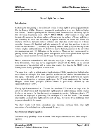
NEUBrewStrayLightCorrection.pdfNOAA-EPA Brewer NetworkFile NameFigure 15. Absolute differences at eight wavelengths as a function of slant path ozonecolumn (N 5000 cases).For the same eight wavelengths we show ratios as a function of ozone slant path columnin Figure 16. We see that for large ozone slant path column and longer wavelength,overcorrection occurs and they might be as large as 50-100%. However the irradiance isthen small, so there is no incongruence between Figure 15 and Figure 16. We also seethat for short wavelength the traces do not extend to large slant path ozone column. Thisis because the cut-on wavelength gets longer as the ozone column increases.Figure 16. Relative differences at eight wavelengths as a function of slant path ozonecolumn (N 5000 cases).Created on 6/5/08Prepared by: P. Kiedron, P. Disterhoft and K. LantzPage 16 of 26
NEUBrewNOAA-EPA Brewer NetworkStrayLightCorrection.pdfFile NameFigure 17. Stray light level and cut-on wavelength as a function of slant path ozonecolumn (N 5000 cases).Figure 17 shows how stray light level and cut-on wavelength change with slant pathozone column. It is obvious that the cut-on wavelength increases with slant path column,but it is less obvious why the stray light level decreases.For each case out of 32 we have generated data and Figures 13 through 17. They are notidentical but they tell the same story. We summarize the results with Figure 18 thatshows the average cut-on wavelength and stray light level (SLL) for 32 cases.As expected the stray light level is slightly larger for PM scans than for AM scans and thecut-on wavelengths are longer for PM scans. This summarizes the differences betweenAM and PM scans and the fact that the stray light correction cannot be perfect in ascanning instrument.In Figure 18 we also plotted the results from Table 2 that contains the results of straylight correction statistics run on real field data. The data, obtained from each instrumentwas from 7000 to 15000 scans each. The stray light levels are within the range ofsimulation results and they even correlate with simulation results. The cut-on wavelengthcorrelates very well. The real responsivities from the Brewers that were used in thesimulations are responsible for the correlation. We haven’t used slit scattering functionsfrom the fielded Brewer as they have not been measured, yet. Functions A and B in Fig.1 are from two other Brewers.Additional graphical results from field data stray light corrections for eight instrumentsare presented in the Appendix.Created on 6/5/08Prepared by: P. Kiedron, P. Disterhoft and K. LantzPage 17 of 26
NEUBrewNOAA-EPA Brewer NetworkStrayLightCorrection.pdfFile NameFigure 18. Average stray light level and average cut-on wavelength for eight Brewers, twoslit scatterings, and AM and PM runs.Table 2. Results for eight MKIV BrewersBrewer IDNumber ofUV ScansStray Light FractionAverageCut-on Wavelength cAverageNoise-to-Signalat c 0.5AverageBR 134BR 139BR 140BR 141BR 144BR 146BR 147BR 70.9590.9530.7980.8490.8950.8090.690Created on 6/5/08Prepared by: P. Kiedron, P. Disterhoft and K. LantzPage 18 of 26
NEUBrewNOAA-EPA Brewer NetworkStrayLightCorrection.pdfFile NameReferencesBernhard, G., C.R. Booth, and J.C. Ehramjian, "Supplement to Version 2 data of the National ScienceFoundation s Ultraviolet Radiation Monitoring Network: South Pole," J. Geophys. Res. 109, D21207,doi:10.1029/2004JD004937, 2004Brown, S.W., B.C. Johnson, M.E. Feinholz, M.A. Yarbrough, S. J. Flora, K. R. Lykke and D. K. Clark,”Stray-light correction algorithm for spectrographs,” Metrologia 40, pp. S81–S84, 2003.Kiedron, P.W, L.H. Harrison, J.L. Berndt, J.J. Michalsky, A.F. Beaubien, “Specifications and performanceof UV rotating shadowband spectroradiometer (UV-RSS),” Ultraviolet Ground- and Space-basedMeasurements, Models, and Effects, James R. Slusser; Jay R. Herman; Wei Gao, Editors, ProceedingsSPIE 4482 , 2002Kiedron, P.W.; L. Harrison; J.J. Michalsky, Jr.; J.A. Schlemmer; J.L. Berndt, “Data and signal processingof rotating shadowband spectroradiometer (RSS) data,” Atmospheric Radiation Measurements andApplications in Climate, Joseph A. Shaw, Editors, Proceedings SPIE 4815, pp. 58-72, 2002.Lakkala, K, A. Arola, A. Heikkil, J. Kaurola, T. Koskela, E. Kyrol, A. Lindfors, O. Meinander, A.Tanskanen, J. Grobner, and G. Hulsen, “Quality assurance of the Brewer UV measurements in Finland,”Atmos. Chem. Phys. Discuss., 8, 1415–1455, 2008.Lantz, K. , P. Disterhoft, E. Early, A. Thompson, J. DeLuisi, P. Kiedron, L. Harrison, J. Berndt, W. Mou,T. J. Erhamjian, L. Cabausua, J. Robertson, D. Hayes, J. Slusser, D. Bigelow, G. Janson, A. Beaubian, M.Beaubian, "The 1997 North American Interagency Intercomparison of Ultraviolet MonitoringSpectroradiometers," J. Res. Natl. Inst. Stand. Technol. 107, 19-62, 2002.Seim. T. and S. Prydz, “Automated spectroradiometer applying computer analysis of spectral data,” Appl.Opt. 11, 5, 1169-1177, 1972.Zong, Y., S.W. Brown., B.C. Johnson, K.R. Lykke, and Y. Ohno,” Simple spectral stray light correctionmethod for array spectroradiometers,” Appl. Opt. 45, 6, pp. 1111-1119, 2006.Appendix: Results for individual instrumentsGraph 1 (1st from the top) shows values of stray light level for each processed scan as afunction of airmass.Graph 2 (2nd from the top) shows the cut-on wavelength for each processed scan as afunction of airmass.Graph 3 (3rd from the top) shows a histogram of noise-to-signal for the cut-onewavelength plus 0.5nm.Created on 6/5/08Prepared by: P. Kiedron, P. Disterhoft and K. LantzPage 19 of 26
NEUBrewStrayLightCorrection.pdfCreated on 6/5/08Prepared by: P. Kiedron, P. Disterhoft and K. LantzNOAA-EPA Brewer NetworkFile NamePage 20 of 26
NEUBrewStrayLightCorrection.pdfCreated on 6/5/08Prepared by: P. Kiedron, P. Disterhoft and K. LantzNOAA-EPA Brewer NetworkFile NamePage 21 of 26
NEUBrewStrayLightCorrection.pdfCreated on 6/5/08Prepared by: P. Kiedron, P. Disterhoft and K. LantzNOAA-EPA Brewer NetworkFile NamePage 22 of 26
NEUBrewStrayLightCorrection.pdfCreated on 6/5/08Prepared by: P. Kiedron, P. Disterhoft and K. LantzNOAA-EPA Brewer NetworkFile NamePage 23 of 26
NEUB
Stray light in the UV scan is a dominant component of the signal C(p) at the shortest wavelengths. Thus the level of stray light can be estimated directly in each UV scan and its value is C(p) at