Transcription
VIIRS DNB SDR Algorithm ImprovementsSteve MillsNOAA STAR/ERT9 August 2016
Subtopics1. Cal based gain ratios and stray lightcorrection2. DNB Offset & Noise Analysis from Cal Data3. Determining offsets using Earth view—astatistical method using a parametric modelwith method of moments estimator Page 2
Part 1 –Cal based gain ratios and stray lightcorrection
Cal Sector Data around Night to Day Transition In theory the cal space-view (SV), blackbody (BB) calibration (cal)should always be dark throughout the orbit.– Space has very little light except for stars and airglow in the ionosphere– The blackbody is black, meaning that it should not reflect any light In fact, both the SV and the BB are affected by stray light– They have strong signals during the day and around both terminator crossing.– This stray light is correlated with the stray light seen in the earth-view (EV) The stray light has been shown to be dependent on satellite solarzenith angle (SSZA) and satellite solar azimuth angle (SSAA)– during the night to day transition in the southern hemisphere the stray light isquite different from the northern hemisphere because of the SSAA is in theopposite direction.– There is a seasonal change in the SSAA over the orbit and so the stray lightchanges from month to month. The solar diffuser (SD) cal sector data is almost always the strongest– This is not surprising since the SD has almost 100% reflectance– Even when the sun is not directly illuminating the SD it apparently is beingilluminated by earthshine throughout the twilight, daytime and even nighttime.
EV “Stray light” around night-to-dayterminator crossingDNB radiance from 07 July 2013 at 13:26 UTC. Thescene is in the southern Pacific off the coast of Antarctica.No stray lightType 1 stray lightType 2 “stray light” Page 5
Comparing SD, SV and EV signals during night to daytransition in southern hemisphereSD low gain stage (LGS)SD mid gain stage (MGS)SV high gain stage (HGS)HGAHGBEV from start of scan Page 6
Comparing SD, SV and EV signals during southernhemisphere terminator crossingType 1Type 2HGAHGBOriginally identifiedas SD stray light Page 7
Comparing SD, SV and EV signals during southernhemisphere terminator crossingAbrupt increase inSV and EV when SDillumination beginsHGAHGB Page 8
Comparing SD, SV and EV signals during southernhemisphere terminator crossingSaw tooth patternHGAHGB Page 9
Comparing SD, SV and EV signals during southernhemisphere terminator crossingSD increases by 2000%Response almost flatHGAHGBOnset of twilight Page 10
Comparing SD, SV and EV signals during southernhemisphere terminator crossingOrder of magnitudedifference in responseHGAHGB Page 11
SV signal during this periodRapid decrease insignal over 0.7 ExtrapolationLinear EV 0 DNExponential EV .03 DNBy itself this effectcould be explained asintense stray light9.5 to EV Page 12
Inconsistencies with stray light hypothesis—What is really going on? Alternative hypothesis—hysteresis from intense SD signal–There are known to be problems with the S-NPP VIIRS DNB anti-blooming electronics–Other mechanisms are possible, e.g. some super-saturation effect in the HGS CCDFact 1: HGS SV & EV signals abruptly start and end over the direct solarillumination of the SD– Fact 2: Saw tooth pattern on HGS SV related to aggregation mode– Possible cause: because the SV signal rapidly decreases & the with lower aggregation there is lesstime per sample, the overall decrease is less with less aggregationFact 3: SV & EV HGS signals otherwise uncorrelated with SD signal but instead havea flat response– Possible cause: anti-blooming circuit abruptly triggered with rapid increase in SD radiancePossible cause: anti-blooming trigger causes an excess charge that is fixed and thus causing offsetsFact 4: EV signal is order of magnitude les than SV mean–Possible cause: Excess charge is rapidly discharged for every sample of SV and continues after the 16samples that are transmitted Page 13
How does this effect “stray light” correction? The type 2 “straylight” offsetcorrection workswell over most ofthe area. In the currentalgorithm theonset of type 2stray light usesthe solar anglewith respect tothe satellite. The onset prediction often is off by up to 3 scans, leaving either a dark orlight streak from under-correction or over-correction. A better predictor would be to use the SD signal with a threshold. Thethreshold of 0.06 mW cm-2 steradian-1 was used to test this. Page 14
Using a SD threshold to predict the SV and EV onsetHGAHGBHysteresis onsetpredictor Page 15
Hysteresis affect on gain ratios from SV or BB For the SD the HGA & HGB signals are almost always saturated and it is rare that MGS/HGSgain ratios can be produced (4 to 5 scans per orbit). Therefore RSBAutoCal currently uses MGS/HGS gain ratios from the SV and BB signal. Since the SV & BB should ideally have no signal, almost all the observed signal must be straylight or hysteresis. The validity of these gain ratios is based on the assumption that the stray light equallyilluminates both MGS and HGS.–There is evidence that this is not true, even on average. During the daytime the EV signal is as strong as or stronger than the SD signal during solarillumination. The BB HGS signal is therefore likely to also be affected by hysteresis during daytime. If some of the BB or DV signal is hysteresis then it is not even optical, so this furtherinvalidates using SV or BB for gain ratios. Therefore, the SV and BB signals should never be used for cross-calibration.–Automatic cross-calibration for MGS/HGS is therefore not possible.–Automatic cross-calibration using the SD for LGS/MGS gain ratios should still be effective Page 16
SV MGS/HGB cross-calibrationHysteresis EffectHysteresis &Stray LightEffectsGain ratio thresholdSNR(MGS) 15 Page 17
BB MGS/HGB cross-calibrationGain ratio thresholdSNR(MGS) 15 Page 18
SD MGS/HGA cross-calibrationGain ratio thresholdSNR(MGS) 15 Page 19
SD LGS/MGS day-to-night cross-calibrationSpread due tonoise &nonlinearityGain ratiothresholdSNR(LGS) 15Stableover orbit Page 20
Conclusions & Recommendations What was previously thought to be stray light from direct sunlight on the SD isactually a hysteresis effect– The cause is unknown but it may be related to anti-blooming in the HGS The hysteresis affects the SV cal signal about an order of magnitude more than theEV– It rapidly decreases over the 16 cal samples– The rapid decrease explains a saw tooth pattern in the SV that is associated with the 72 scanDNB cal cycle The onset of the effect for the SV and EV is abrupt after which it immediately goesto a flat responsePrediction of the onset has always been a problem for the stray light correction,but using a simple threshold on the SD signal onset can be predicted to within onescan.It is likely that the BB cal signal is also impacted by hysteresis from the EV duringthe daytime.Hysteresis adversely affects gain ratios derived from the SV or BB.– Large uncertainties ( 50%) are probably due to hysteresis and uneven stray light illumination. RSBAutoCal should not use the SV or BB to produce gain ratiosProbably there is no reliable way to automatically produce MGS/HGS gain ratios Page 21
Part 1—Backup
SV MGS/HGA cross-calibrationHysteresis EffectHysteresis &Stray LightEffectsGain ratio thresholdSNR(MGS) 15 Page 23
BB MGS/HGA cross-calibrationGain ratio thresholdSNR(MGS) 15 Page 24
SD MGS/HGB cross-calibrationGain ratio thresholdSNR(MGS) 15 Page 25
Part 2—DNB Offset & Noise Analysisfrom Cal Data
DNB Offset using cal data Because of fixed pattern offsets in the EV, the cal sectordata cannot be used to determine absolute offset It has been proposed that dark cal data can be used fortracking the relative change in dark offset– This has not been demonstrated to be true for all agg modes Rather than replicate what has already been done I try todevelop a statistically rigorous method for determiningthese offset along with the dark noise In particular, evaluation of fixed pattern offset in the calsamples and method for outlier removal are considered
Will use a statistically rigorous methodology Page 28
Fixed Pattern Offset (FPO) Dominates HGA CalHGA Fixed Pattern Offsets for 4 aggregations. Solid lines are offsets, dotted lines aredifferences plotted to show noise level. Both HAM sides are plotted with " " for side 0 and "x"for side 1. Color indicates detector number. Page 29
Fixed Pattern Offset Dominates MGS CalMGS Fixed Pattern Offsets for 4 aggregations. Solid lines are offsets, dotted lines are differencesplotted to show noise level. Both HAM sides are plotted with " " for side 0 and "x" for side 1. Colorindicates detector number. Page 30
Fixed Pattern Offset Dominates LGS CalLGS Fixed Pattern Offsets for 4 aggregations. Solid lines are offsets, dotted lines are differencesplotted to show noise level. Both HAM sides are plotted with " " for side 0 and "x" for side 1. Colorindicates detector number. Page 31
Difference in Means, HG SV-BBIncrease due to airglow in ionosphere limb Page 32
Difference in Means, HG SD-BBNew MoonSmall bias on SD due to faint light (e.g. airglow) from earth Page 33
Difference in Means, HG SD-BBFull MoonLarge bias on SD due to moonlight from earth Page 34
Detector noise and FPO variation compared for HGAFPO variation dominates in the samples Page 35
Noise Equivalent Radiance (NER) by Aggregation Page 36
Methods of Outlier Mitigation (1 of 2) Winsorization –This method does not require taking the mean or themedian and uses the entire ensemble to identify outliers.– It takes as parameters the maximum and minimum percentile of data outside of whichare to be treated as outliers, for example, the lowest 2% and highest 2%.– Any data that is identified within the lowest range is replaced with the value exactly atthe lowest cutoff point.– Likewise, data that is identified within the highest range is replaced with the valueexactly at the highest cutoff point.– Because it replaces the data rather than remove it, the resulting ensemble has the samenumber of elements as the input ensemble. Trimming—This is similar to winsorization except that it removes, ratherthan replaces, the data below or above the percentile limits.– Like winsorization it takes as parameters the maximum and minimum percentile of dataoutside of which are to be treated as outliers,– but instead of replacing these values it trims these data elements from the ensemble.– The resulting ensemble has fewer elements than the input ensemble. Page 37
Methods of Outlier Mitigation (2 of 2) Page 38
Conclusions & Recommendations (1 of 3) The cal data may be useful in determining offset drift in the EV.– Because of the high uncertainty in the offsets derived from earth view data it is notcertain whether in fact the drifts always correlate.– It has been shown that they approximately correlate for at least some detectors andAgg. Seq., but this has not been shown to be true in general. The BB is the best cal data to use for offset determination and for noiseestimation because it is not strongly contaminated by indirect light fromthe earth or by airglow, unlike the SD and SV.– Even for the MGS, during a full moon there is sufficient light to produce a detectableoffset in SD, and likewise for airglow contamination in the SV.– Also, including SV and SD only adds an unnecessary level of complexity to the analysisand at worst may reduce the accuracy. Because of FPO data ensemble averages should always be taken over thesame sample over many scans– Per scan averages should never be taken– Outlier removal should be done on per sample ensembles, and never per scan Page 39
Conclusions & Recommendations (2 of 3) FPO is a function of sample number, detector number, Agg. Seq. and gain stage,but is not apparently a function of HAM side or cal source. To determine NEC without the effect of FPO, data with the same sample number,detector number, Agg. Seq. and gain stage can be subtracted, and the standarddeviation taken. NEC determined in this way was found for:–HGA and HGB to go from 1.75 DN for Agg. Seq. 1 to 3.3 DN for Agg. Seq. 32.–MGS NEC 1.01 DN for all Agg. Seq.–LGS NEC 0.74 DN for all Agg. Seq. After eliminating data effected by solar stray light using the solar nadir angle, thereare about 10,000 samples per day for each detector, HAM side, Agg Seq. and gainstage combination. This number of samples is sufficient to determine offset drift for for the daily mean–high-gain Agg. Seq. 32 to within a HGS uncertainty 0.03 DN.–MGS and LGS the uncertainty 0.01 DN. Page 40
Conclusions & Recommendations (3 of 3) The method used for outlier mitigation has a large impact on the uncertainty ofthe daily mean offset as well as the NEC.–Modeling showed that Winsorization had the least impact on uncertainty, and this is the process thatis recommended here.–Trimming and Multilayer Median Trimming were also considered but did not perform as well.More important than the method used for outlier mitigation is the limits used.–These should not be arbitrarily set but should be set by first determining the probability of outliersthat are mostly due to HEP hits.–It is recommended that this probability should be determined using either Peirce’s criterion and/orChauvenet's criterion to identify likely outliers.There may be sufficient indirect light during a full moon to produce a detectiblesignal in the daily mean offsets from BB.– These events should be studied and if necessary removed from the trending using a threshold lunarphase.Outlier processing should also be performed on the daily mean offsets afterremoving the impact of drift.–This may be need to remove anomalous events that occur over a period longer than a few seconds. Page 41
Part2—Backup
DNB Cal Data Form As with all the other bands on VIIRS, the DNB views the space view (SV),black body (BB) and solar diffuser (SD) calibration (cal) views one per scan.There are two differences regarding the DNB functionality compared withthe other bands: It has 4 gain stages, HGA, HGB, MGS and LGS, compared with 1 or 2 stagescompared with the other bands; It has 32 aggregation modes plus 4 diagnostic aggregation modescompared with 3 aggregation modes for the other bands. To accommodate these differences, the DNB cal data are acquireddifferently. The features of the data that are different are: There are only 16 samples per scan per gain stage for DNB (compared with48 for Moderate Resolution bands and 96 for imagery bands). The aggregation modes cycle through every 72 scans with 2 scans for eachmode (one for each HAM side). Aggregation modes are numbered from the center at 1 to the edge at 32 Aggregation sequences are numbered from the edge at 1 to the center at32
Rate of Offset Change ComparisonDet 1 HAM AAgg 12Agg 32Top: HGS rate of change fitted from 47 new moon days(02/21/2012 and 46 days between 11/13/2012 and07/04/2016).Cal view data: follow the RSBAutoCal algorithm todetermine DNB dark signal.Earth view data (VROP): DNB DN0 LUT (HGS)Middle: relative difference of the fitted change of rate(rate CalView - rate EarthView)/rate EarthView.Bottom: zoomed in figure of the middle figure
Fixed Pattern Offset Dominates HGB CalHGB Fixed Pattern Offsets for 4 aggregations. Solid lines are offsets, dotted lines are differencesplotted to show noise level. Both HAM sides are plotted with " " for side 0 and "x" for side 1. Colorindicates detector number. Page 45
Detector noise and FPO variation compared for HGBFPO variation for HGB is different from HGA, but it usuallydominates for lower Aggregation Sequence Number Page 46
HGA & HGB Dark Noise Equivalent Counts(NEC) Computed 8 Ways Cal cycle SV difference is large due to airglow variation and long time span HAM SV likely has higher NEC due to airglow variation Page 47
Part 3—Determining offsets using Earth view—astatistical method using a parametric model withmethod of moments estimator Page 48
Summary of methodology The primary method for determining dark offset is to view theearth at night over the Pacific during a new moon but even without any lunar illumination, there is always somedetectable light coming from the earth. This makes it difficult to use dark earth view data todetermine offset tables that are not biased. What is proposed here is to use a statistical estimator and aparametric model of the natural illumination to determine thelevel of natural illumination and therefore correct for it. I considered for this are Maximum Likelihood Estimation(MLE) and the Method of Moments Estimation (MME). Here only MME will be considered, but it would beworthwhile to investigate MLE. Page 49
What data to use When determining the MGS and LGS offsets only the data fromVROP 702 and 705 are available to be used, but for HGS this is not arestriction. The HGS offset data has always been taken over the Pacific Oceanon the day of the new moon, but is it really necessary to restrict thedata to only these exact new moon dates? The reason for using the Pacific is because there is very few fixedlights, but this is just as true for the Indian Ocean or most of theAtlantic Ocean. Also there are places on land such as the Sahara Desert which aresimilarly deplete of fixed light. Because there are databases that provide data on persistent lightover the entire earth, recommend that rather than restricting thedata collection to certain regions, it is better to use all data andthen filter out pixels where there are persistent lights based on thegeolocation of the pixels. Page 50
Ocean With no lunar illuminationWeak air glowStronger airglowHGS granule taken on 22 Sep 2014 between 11:47:052 and 11:52:46 UTC, during a new moon in the region overthe South Pacific Ocean. The plotting range from black to white is from -8.3 10-11 to 4.2 10-10 W cm-2 str-1. Page 51
Distributions from new moon DNB scenesDistribution shapechanges withaggregation zone.More skew nearnadir. Page 52
Math model for scene radianceTypes of illumination: Unnatural nighttime illumination (UNI) includes electrical lights, gas flares andother anthropogenic fires.Natural Nighttime Illumination (NNI):– extraterrestrial nighttime illumination (ETI), including stars, zodiacal light and planets.– Airglow, both direct and reflected.– natural terrestrial sources other than airglow, including the Aurora Borealis, Aurora Australis,lightning, algae blooms and natural fires.Remove through filtering
Equate sensor response to scene radiance model Page 54
Produce simultaneous equations using 1st, 2nd & 3rdmoments (mean, variance & skew) Page 55
Conclusions Because of the statistical nature of the sensor noiseand scene radiance, a statistical estimator seems tobe the only way to solve this problem More work is needed to develop this methodology The math is complicated but it should not be difficultto program in a language such as Python or IDL. In addition to providing unbiased offsets, thismethod would also provide a mathematical modelfor understanding airglow distribution Page 56
How does this effect “stray light” correction? The type 2 “stray light” offset correction works well over most of the area. In the current algorithm the onset of type 2 stray light uses the solar angle with re