Transcription
G * Power 3.1 manualJanuary 21, 2021This manual is not yet complete. We will be adding help on more tests in the future. If you cannot find help for your testin this version of the manual, then please check the G*Power website to see if a more up-to-date version of the manualhas been made available.Contents21 t test: Means - difference between two independentmeans (two groups)521Introduction22The G * Power calculator73Exact: Correlation - Difference from constant (onesample case)922 Wilcoxon signed-rank test: Means - difference fromconstant (one sample case)5323 Wilcoxon signed-rank test: (matched pairs)4Exact: Proportion - difference from constant (onesample case)115Exact: Proportion - inequality, two dependentgroups (McNemar)146Exact: Proportions - inequality of two independentgroups (Fisher’s exact-test)175524 Wilcoxon-Mann-Whitney test of a difference between two independent means5925 t test: Generic case6326 χ2 test: Variance - difference from constant (onesample case)6427 z test: Correlation - inequality of two independentPearson r’s657Exact test: Multiple Regression - random model188Exact: Proportion - sign test2228 z test: Correlation - inequality of two dependentPearson r’s669Exact: Generic binomial test2329 Z test: Multiple Logistic Regression702430 Z test: Poisson Regression7531 Z test: Tetrachoric Correlation80References8410 F test: Fixed effects ANOVA - one way11 F test: Fixed effects ANOVA - special, main effectsand interactions2612 t test: Linear Regression (size of slope, one group) 3113 F test: Multiple Regression - omnibus (deviation ofR2 from zero), fixed model3314 F test: Multiple Regression - special (increase ofR2 ), fixed model3615 F test: Inequality of two Variances3916 t test: Correlation - point biserial model4017 t test: Linear Regression (two groups)4218 t test: Linear Regression (two groups)4519 t test: Means - difference between two dependentmeans (matched pairs)4820 t test: Means - difference from constant (one sample case)501
1IntroductionDistribution-based approach to test selection First selectthe family of the test statistic (i.e., exact, F , t , χ2 , or ztest) using the Test family menu in the main window. TheStatistical test menu adapts accordingly, showing a list of alltests available for the test family.G * Power (Fig. 1 shows the main window of the program)covers statistical power analyses for many different statistical tests of the F test,Example: For the two groups t-test, first select the test familybased on the t distribution. t test, χ2 -test and z test families and some exact tests.G * Power provides effect size calculators and graphicsoptions. G * Power supports both a distribution-based anda design-based input mode. It contains also a calculator thatsupports many central and noncentral probability distributions.G * Power is free software and available for Mac OS Xand Windows XP/Vista/7/8.1.1Then select Means: Difference between two independent means(two groups) option in the Statictical test menu.Types of analysisG * Power offers five different types of statistical poweranalysis:1. A priori (sample size N is computed as a function ofpower level 1 β, significance level α, and the to-bedetected population effect size)2. Compromise (both α and 1 β are computed as functions of effect size, N, and an error probability ratioq β/α)3. Criterion (α and the associated decision criterion arecomputed as a function of 1 β, the effect size, and N)Design-based approach to the test selection Alternatively, one might use the design-based approach. With theTests pull-down menu in the top row it is possible to select4. Post-hoc (1 β is computed as a function of α, the population effect size, and N) the parameter class the statistical test refers to (i.e.,correlations and regression coefficients, means, proportions, or variances), and5. Sensitivity (population effect size is computed as afunction of α, 1 β, and N)1.2 the design of the study (e.g., number of groups, independent vs. dependent samples, etc.).Program handlingPerform a Power Analysis Using G * Power typically involves the following three steps:The design-based approach has the advantage that test options referring to the same parameter class (e.g., means) arelocated in close proximity, whereas they may be scatteredacross different distribution families in the distributionbased approach.1. Select the statistical test appropriate for your problem.2. Choose one of the five types of power analysis available3. Provide the input parameters required for the analysisand click "Calculate".Example: In the Tests menu, select Means, then select Two independent groups" to specify the two-groups t test.Plot parameters In order to help you explore the parameter space relevant to your power analysis, one parameter(α, power (1 β), effect size, or sample size) can be plottedas a function of another parameter.1.2.1Select the statistical test appropriate for your problemIn Step 1, the statistical test is chosen using the distributionbased or the design-based approach.2
Figure 1: The main window of G * Power1.2.2 the required power level (1 β),Choose one of the five types of power analysisavailable the pre-specified significance level α, andIn Step 2, the Type of power analysis menu in the center ofthe main window is used to choose the appropriate analysistype and the input and output parameters in the windowchange accordingly. the population effect size to be detected with probability (1 β).In a criterion power analysis, α (and the associated decision criterion) is computed as a function ofExample: If you choose the first item from the Type of poweranalysis menu the main window will display input and outputparameters appropriate for an a priori power analysis (for t testsfor independent groups if you followed the example providedin Step 1). 1-β, the effect size, and a given sample size.In a compromise power analysis both α and 1 β arecomputed as functions of the effect size, N, and an error probability ratio q β/α.In a post-hoc power analysis the power (1 β) is computed as a function ofIn an a priori power analysis, sample size N is computedas a function of3
α,Because Cohen’s book on power analysis Cohen (1988)appears to be well known in the social and behavioral sciences, we made use of his effect size measures wheneverpossible. In addition, wherever available G * Power provides his definitions of "‘small"’, "‘medium"’, and "‘large"’effects as "‘Tool tips"’. The tool tips may be optained bymoving the cursor over the "‘effect size"’ input parameterfield (see below). However, note that these conventions mayhave different meanings for different tests. the population effect size parameter, and the sample size(s) used in a study.In a sensitivity power analysis the critical population effect size is computed as a function of α, 1 β, andExample: The tooltip showing Cohen’s measures for the effectsize d used in the two groups t test N.1.2.3Provide the input parameters required for the analysisIn Step 3, you specify the power analysis input parametersin the lower left of the main window.Example: An a priori power analysis for a two groups t testwould require a decision between a one-tailed and a two-tailedtest, a specification of Cohen’s (1988) effect size measure d under H1 , the significance level α, the required power (1 β) ofthe test, and the preferred group size allocation ratio n2 /n1 .Let us specify input parameters forIf you are not familiar with Cohen’s measures, if youthink they are inadequate for your test problem, or if youhave more detailed information about the size of the to-beexpected effect (e.g., the results of similar prior studies),then you may want to compute Cohen’s measures frommore basic parameters. In this case, click on the Determinebutton to the left the effect size input field. A drawer willopen next to the main window and provide access to aneffect size calculator tailored to the selected test. a one-tailed t test, a medium effect size of d .5, α .05, (1 β) .95, and an allocation ratio of n2 /n1 1Example: For the two-group t-test users can, for instance, specify the means µ1 , µ2 and the common standard deviation (σ σ1 σ2 ) in the populations underlying the groups to calculate Cohen’s d µ1 µ2 /σ. Clicking the Calculate andtransfer to main window button copies the computed effectsize to the appropriate field in the main windowThis would result in a total sample size of N 176 (i.e., 88observation units in each group). The noncentrality parameterδ defining the t distribution under H1 , the decision criterionto be used (i.e., the critical value of the t statistic), the degreesof freedom of the t test and the actual power value are alsodisplayed.In addition to the numerical output, G * Power displaysthe central (H0 ) and the noncentral (H1 ) test statistic distributions along with the decision criterion and the associatederror probabilities in the upper part of the main window.This supports understanding the effects of the input parameters and is likely to be a useful visualization tool inNote that the actual power will often be slightly largerthan the pre-specified power in a priori power analyses. Thereason is that non-integer sample sizes are always roundedup by G * Power to obtain integer values consistent with apower level not less than the pre-specified one.4
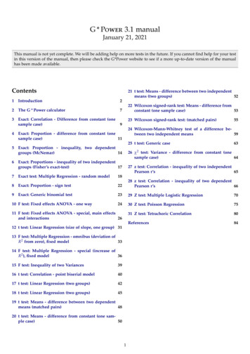
pendent variable y. In an a prior analysis, for instance, thisis the sample size.the teaching of, or the learning about, inferential statistics.The distributions plot may be copied, saved, or printed byclicking the right mouse button inside the plot area.The button X-Y plot for a range of values at to bottom ofthe main window opens the plot window.Example: The menu appearing in the distribution plot for thet-test after right clicking into the plot.By selecting the appropriate parameters for the y and thex axis, one parameter (α, power (1 β), effect size, or sample size) can be plotted as a function of another parameter. Of the remaining two parameters, one can be chosen todraw a family of graphs, while the fourth parameter is keptconstant. For instance, power (1 β) can be drawn as afunction of the sample size for several different populationeffects sizes, keeping α at a particular value.The plot may be printed, saved, or copied by clicking theright mouse button inside the plot area.Selecting the Table tab reveals the data underlying theplot (see Fig. 3); they may be copied to other applicationsby selecting, cut and paste.The input and output of each power calculation in aG*Power session are automatically written to a protocolthat can be displayed by selecting the "Protocol of poweranalyses" tab in the main window. You can clear the protocol, or to save, print, and copy the protocol in the same wayas the distributions plot.Note: The Power Plot window inherits all input parameters of the analysis that is active when the X-Y plotfor a range of values button is pressed. Only someof these parameters can be directly manipulated in thePower Plot window. For instance, switching from a plotof a two-tailed test to that of a one-tailed test requireschoosing the Tail(s): one option in the main window, followed by pressing the X-Y plot for range of values button.(Part of) the protocol window.1.2.4Plotting of parametersG * Power provides to possibility to generate plots of oneof the parameters α, effectsize, power and sample size, depending on a range of values of the remaining parameters.The Power Plot window (see Fig. 2) is opened by clicking the X-Y plot for a range of values button locatedin the lower right corner of the main window. To ensurethat all relevant parameters have valid values, this button isonly enabled if an analysis has successfully been computed(by clicking on calculate).The main output parameter of the type of analysis selected in the main window is by default selected as the de-5
Figure 2: The plot window of G * PowerFigure 3: The table view of the data for the graphs shown in Fig. 26
2The G * Power calculator sign(x) - Sign of x: x 0 1, x 0 0, x 0 1.G * Power contains a simple but powerful calculator thatcan be opened by selecting the menu label "Calculator" inthe main window. Figure 4 shows an example session. Thissmall example script calculates the power for the one-tailedt test for matched pairs and demonstrates most of the available features: lngamma(x) Natural logarithm of the gamma functionln(Γ( x )) frac(x) - Fractional part of floating point x: frac(1.56)is 0.56. int(x) - Integer part of float point x: int(1.56) is 1. There can be any number of expressions min(x,y) - Minimum of x and y The result is set to the value of the last expression inthe script max(x,y) - Maximum of x and y Several expression on a line are separated by a semicolon uround(x,m) - round x up to a multiple of muround(2.3, 1) is 3, uround(2.3, 2) 4. Expressions can be assigned to variables that can beused in following expressionsSupported distribution functions (CDF cumulativedistribution function, PDF probability density function, Quantile inverse of the CDF). For information about the properties of these distributions checkhttp://mathworld.wolfram.com/. The character # starts a comment. The rest of the linefollowing # is ignored Many standard mathematical functions like squareroot, sin, cos etc are supported (for a list, see below) zcdf(x) - CDFzpdf(x) - PDFzinv(p) - Quantileof the standard normal distribution. Many important statistical distributions are supported(see list below) normcdf(x,m,s) - CDFnormpdf(x,m,s) - PDFnorminv(p,m,s) - Quantileof the normal distribution with mean m and standarddeviation s. The script can be easily saved and loaded. In this waya number of useful helper scripts can be created.The calculator supports the following arithmetic operations (shown in descending precedence): Power: Multiply: Divide: / Plus: Minus: - chi2cdf(x,df) - CDFchi2pdf(x,df) - PDFchi2inv(p,df) - Quantileof the chi square distribution with d f degrees of freedom: χ2d f ( x ).(2 3 8)(2 2 4)(6/2 3)(2 3 5) fcdf(x,df1,df2) - CDFfpdf(x,df1,df2) - PDFfinv(p,df1,df2) - Quantileof the F distribution with d f 1 numerator and d f 2 denominator degrees of freedom Fd f1 ,d f2 ( x ).(3 2 1)Supported general functions abs(x) - Absolute value x tcdf(x,df) - CDFtpdf(x,df) - PDFtinv(p,df) - Quantileof the Student t distribution with d f degrees of freedom td f ( x ). sin(x) - Sine of x asin(x) - Arc sine of x cos(x) - Cosine of x acos(x) - Arc cosine of x ncx2cdf(x,df,nc) - CDFncx2pdf(x,df,nc) - PDFncx2inv(p,df,nc) - Quantileof noncentral chi square distribution with d f degreesof freedom and noncentrality parameter nc. tan(x) - Tangent of x atan(x) - Arc tangent of x atan2(x,y) - Arc tangent of y/x ncfcdf(x,df1,df2,nc) - CDFncfpdf(x,df1,df2,nc) - PDFncfinv(p,df1,df2,nc) - Quantileof noncentral F distribution with d f 1 numerator andd f 2 denominator degrees of freedom and noncentralityparameter nc. exp(x) - Exponential e x log(x) - Natural logarithm ln( x ) sqrt(x) - Square root x sqr(x) - Square x27
Figure 4: The G * Power calculator mr2cdf(R2 , ρ2 ,k,N) - CDFmr2pdf(R2 , ρ2 ,k,N) - PDFmr2inv(p,ρ2 ,k,N) - Quantileof the distribution of the sample squared multiple correlation coefficient R2 for population squared multiplecorrelation coefficient ρ2 , k 1 predictors, and samplesof size N. nctcdf(x,df,nc) - CDFnctpdf(x,df,nc) - PDFnctinv(p,df,nc) - Quantileof noncentral Student t distribution with d f degrees offreedom and noncentrality parameter nc. betacdf(x,a,b) - CDFbetapdf(x,a,b) - PDFbetainv(p,a,b) - Quantileof the beta distribution with shape parameters a and b. logncdf(x,m,s) - CDFlognpdf(x,m,s) - PDFlogninv(p,m,s) - Quantileof the log-normal distribution, where m, s denote meanand standard deviation of the associated normal distribution. poisscdf(x,λ) - CDFpoisspdf(x,λ) - PDFpoissinv(p,λ) - Quantilepoissmean(x,λ) - Meanof the poisson distribution with mean λ. laplcdf(x,m,s) - CDFlaplpdf(x,m,s) - PDFlaplinv(p,m,s) - Quantileof the Laplace distribution, where m, s denote locationand scale parameter. binocdf(x,N,π) - CDFbinopdf(x,N,π) - PDFbinoinv(p,N,π) - Quantileof the binomial distribution for sample size N and success probability π. expcdf(x,λ - CDFexppdf(x,λ) - PDFexpinv(p,λ - Quantileof the exponential distribution with parameter λ. hygecdf(x,N,ns,nt) - CDFhygepdf(x,N,ns,nt) - PDFhygeinv(p,N,ns,nt) - Quantileof the hypergeometric distribution for samples of sizeN from a population of total size nt with ns successes. unicdf(x,a,b) - CDFunipdf(x,a,b) - PDFuniinv(p,a,b) - Quantileof the uniform distribution in the intervall [ a, b]. corrcdf(r,ρ,N) - CDFcorrpdf(r,ρ,N) - PDFcorrinv(p,ρ,N) - Quantileof the distribution of the sample correlation coefficientr for population correlation ρ and samples of size N.8
3Exact: Correlation - Difference fromconstant (one sample case)asymptotically identical, that is, they produce essentially the same results if N is large. Therefore, a threshold value x for N can be specified that determines thetransition between both procedures. The exact procedure is used if N x, the approximation otherwise.The null hypothesis is that in the population the true correlation ρ between two bivariate normally distributed random variables has the fixed value ρ0 . The (two-sided) alternative hypothesis is that the correlation coefficient has adifferent value: ρ 6 ρ0 :H0 :H1 :2. Use large sample approximation (Fisher Z). With this option you select always to use the approximation.There are two properties of the output that can be usedto discern which of the procedures was actually used: Theoption field of the output in the protocol, and the namingof the critical values in the main window, in the distributionplot, and in the protocol (r is used for the exact distributionand z for the approximation).ρ ρ0 0ρ ρ0 6 0.A common special case is ρ0 0 (see e.g. Cohen, 1969,Chap. 3). The two-sided test (“two tails”) should be usedif there is no restriction on the direction of the deviationof the sample r from ρ0 . Otherwise use the one-sided test(“one tail”).3.13.3In the null hypothesis we assume ρ0 0.60 to be the correlation coefficient in the population. We further assume thatour treatment increases the correlation to ρ 0.65. If werequire α β 0.05, how many subjects do we need in atwo-sided test?Effect size indexTo specify the effect size, the conjectured alternative correlation coefficient ρ should be given. ρ must conform to thefollowing restrictions: 1 ε ρ 1 ε, with ε 10 6 .The proper effect size is the difference between ρ and ρ0 :ρ ρ0 . Zero effect sizes are not allowed in a priori analyses.G * Power therefore imposes the additional restriction that ρ ρ0 ε in this case.For the special case ρ0 0, Cohen (1969, p.76) defines thefollowing effect size conventions: SelectType of power analysis: A priori OptionsUse exact distribution if N : 10000 InputTail(s): TwoCorrelation ρ H1: 0.65α err prob: 0.05Power (1-β err prob): 0.95Correlation ρ H0: 0.60 small ρ 0.1 medium ρ 0.3 large ρ 0.5Pressing the Determine button on the left side of the effect size label opens the effect size drawer (see Fig. 5). Youcan use it to calculate ρ from the coefficient of determination r2 . OutputLower critical r: 0.570748Upper critical r: 0.627920Total sample size: 1928Actual power: 0.950028In this case we would reject the null hypothesis if we observed a sample correlation coefficient outside the interval [0.571, 0.627]. The total sample size required to ensurea power (1 β) 0.95 is 1928; the actual power for this Nis 0.950028.In the example just discussed, using the large sample approximation leads to almost the same sample size N 1929. Actually, the approximation is very good in mostcases. We now consider a small sample case, where thedeviation is more pronounced: In a post hoc analysis ofa two-sided test with ρ0 0.8, ρ 0.3, sample size 8, andα 0.05 the exact power is 0.482927. The approximationgives the slightly lower value 0.422599.Figure 5: Effect size dialog to determine the coefficient of determination from the correlation coefficient ρ.3.2ExamplesOptionsThe procedure uses either the exact distribution of the correlation coefficient or a large sample approximation basedon the z distribution. The options dialog offers the following choices:3.4Related testsSimilar tests in G * Power 3.0:1. Use exact distribution if N x. The computation time ofthe exact distribution increases with N, whereas thatof the approximation does not. Both procedures are Correlation: Point biserial model Correlations: Two independent Pearson r’s (two samples)9
3.5Implementation notesExact distribution. The H0 -distribution is the sample correlation coefficient distribution sr (ρ0 , N ), the H1 distribution is sr (ρ, N ), where N denotes the total sample size, ρ0 denotes the value of the baseline correlationassumed in the null hypothesis, and ρ denotes the ‘alternative correlation’. The (implicit) effect size is ρ ρ0 . Thealgorithm described in Barabesi and Greco (2002) is used tocalculate the CDF of the sample coefficient distribution.Large sample approximation. The H0 -distribution is thestandard normal distribution N (0, 1), the H1-distribution isN ( Fz (ρ) Fz (ρ0 ))/σ, 1), with Fz (r )p ln((1 r )/(1 r ))/2(Fisher z transformation) and σ 1/( N 3).3.6ValidationThe results in the special case of ρ0 0 were comparedwith the tabulated values published in Cohen (1969). Theresults in the general case were checked against the valuesproduced by PASS (Hintze, 2006).10
4Exact: Proportion - difference fromconstant (one sample case)The relational value given in the input field on the left sideand the two proportions given in the two input fields on theright side are automatically synchronized if you leave oneof the input fields. You may also press the Sync valuesbutton to synchronize manually.Press the Calculate button to preview the effect size gresulting from your input values. Press the Transfer tomain window button to (1) to calculate the effect size g π π0 P2 P1 and (2) to change, in the main window,the Constant proportion field to P1 and the Effect sizeg field to g as calculated.The problem considered in this case is whether the probability π of an event in a given population has the constantvalue π0 (null hypothesis). The null and the alternative hypothesis can be stated as:H0 :H1 :π π0 0π π0 6 0.A two-tailed binomial tests should be performed to testthis undirected hypothesis. If it is possible to predict a priori the direction of the deviation of sample proportions pfrom π0 , e.g. p π0 0, then a one-tailed binomial testshould be chosen.4.14.2OptionsThe binomial distribution is discrete. It is thus not normallypossible to arrive exactly at the nominal α-level. For twosided tests this leads to the problem how to “distribute” αto the two sides. G * Power offers the three options listedhere, the first option being selected by default:Effect size indexThe effect size g is defined as the deviation from the constant probability π0 , that is, g π π0 .The definition of g implies the following restriction: ε (π0 g) 1 ε. In an a priori analysis we need to respect the additional restriction g ε (this is in accordancewith the general rule that zero effect hypotheses are undefined in a priori analyses). With respect to these constraints,G * Power sets ε 10 6 .Pressing the Determine button on the left side of the effect size label opens the effect size drawer:1. Assign α/2 to both sides: Both sides are handled independently in exactly the same way as in a one-sidedtest. The only difference is that α/2 is used instead ofα. Of the three options offered by G * Power , this oneleads to the greatest deviation from the actual α (in posthoc analyses).2. Assign to minor tail α/2, then rest to major tail (α2 α/2, α1 α α2 ): First α/2 is applied to the side ofthe central distribution that is farther away from thenoncentral distribution (minor tail). The criterion usedfor the other side is then α α1 , where α1 is the actualα found on the minor side. Since α1 α/2 one canconclude that (in post hoc analyses) the sum of the actual values α1 α2 is in general closer to the nominalα-level than it would be if α/2 were assigned to bothside (see Option 1).3. Assign α/2 to both sides, then increase to minimize the difference of α1 α2 to α: The first step is exactly the sameas in Option 1. Then, in the second step, the criticalvalues on both sides of the distribution are increased(using the lower of the two potential incremental αvalues) until the sum of both actual α values is as closeas possible to the nominal α.You can use this dialog to calculate the effect size g fromπ0 (called P1 in the dialog above) and π (called P2 in thedialog above) or from several relations between them. If youopen the effect dialog, the value of P1 is set to the value inthe constant proportion input field in the main window.There are four different ways to specify P2:Press the Options button in the main window to selectone of these options.4.3ExamplesWe assume a constant proportion π0 0.65 in the population and an effect size g 0.15, i.e. π 0.65 0.15 0.8.We want to know the power of a one-sided test givenα .05 and a total sample size of N 20.1. Direct input: Specify P2 in the corresponding input fieldbelow P12. Difference: Choose difference P2-P1 and insert thedifference into the text field on the left side (the difference is identical to g). SelectType of power analysis: Post hoc3. Ratio: Choose ratio P2/P1 and insert the ratio valueinto the text field on the left side OptionsAlpha balancing in two-sided tests: Assign α/2 on bothsides4. Odds ratio: Choose odds ratio and insert the odds ratio ( P2/(1 P2))/( P1/(1 P1)) between P1 and P2into the text field on the left side.11
Figure 6: Distribution plot for the example (see text)would choose N 16 as the result of a search for the sample size that leads to a power of at least 0.3. All types ofpower analyses except post hoc are confronted with similar problems. To ensure that the intended result has beenfound, we recommend to check the results from these typesof power analysis by a power vs. sample size plot. InputTail(s): OneEffect size g: 0.15α err prob: 0.05Total sample size: 20Constant proportion: 0.65 OutputLower critical N: 17Upper critical N: 17Power (1-β err prob): 0.411449Actual α: 0.0443764.4Related testsSimilar tests in G * Power 3.0: Proportions: Sign test.The results show that we should reject the null hypothesis of π 0.65 if in 17 out of the 20 possible cases therelevant event is observed. Using this criterion, the actual αis 0.044, that is, it is slightly lower than the requested α of5%. The power is 0.41.Figure 6 shows the distribution plots for the example. Thered and blue curves show the binomial distribution underH0 and H1 , respectively. The vertical line is positioned atthe critical value N 17. The horizontal portions of thegraph should be interpreted as the top of bars ranging fromN 0.5 to N 0.5 around an integer N, where the heightof the bars correspond to p( N ).We now use the graphics window to plot power values for a range of sample sizes. Press the X-Y plot fora range of values button at the bottom of the main window to open the Power Plot window. We select to plot thepower as a function of total sample size. We choose a rangeof samples sizes from 10 in steps of 1 through to 50. Next,we select to plot just one graph with α 0.05 and effectsize g 0.15. Pressing the Draw Plot button produces theplot shown in Fig. 7. It can be seen that the power does notincrease monotonically but in a zig-zag fashion. This behavior is due to the discrete nature of the binomial distributionthat prevents that arbitrary α value can be realized. Thus,the curve should not be interpreted to show that the powerfor a fixed α sometimes decreases with increasing samplesize. The real reason for the non-monotonic behaviour isthat the actual α level that can be realized deviates more orless from the nominal α level for different sample sizes.This non-monotonic behavior of the power curve poses aproblem if we want to determine, in an a priori analysis, theminimal sample size needed to achieve a certain power. Inthese cases G * Power always tries to find the lowest sample size for which the power is not less than the specifiedvalue. In the case depicted in Fig. 7, for instance, G * Power4.5Implementation notesThe H0 -distribution is the Binomial distribution B( N, π0 ),the H1 -distribution the Binomial distribution B( N, g π0 ).N denotes the total sample size, π0 the constant proportionassumed in the null hypothesis, and g the effect size indexas defined above.4.6ValidationThe results of G * Power for the special case of the sign test,that is π0 0.5, were checked against the tabulated valuesgiven in Cohen (1969, chapter 5). Cohen always chose fromthe realizable α values the one that is closest to the nominalvalue even if it is larger then the nominal value. G * Power, in contrast, always requires the actual α to be lower thenthe nominal value. In cases where the α value chosen byCohen happens to be lower then the nominal α, the resultscomputed with G * Power were very similar to the tabulated values. In the other cases, the power values computedby G * Power were lower then the tabulated ones.In the general case (π0 6 0.5) the results of post hocanalyses for a number of parameters were checked againstthe results produced by PASS (Hintze, 2006). No differenceswere found in one-sided tests. The results for two-sidedtests were also identical if the alpha balancing method “Assign α/2 to both sides” was chosen in G * Power .12
Figure 7: Plot of power vs.
G*Power provides to possibility to generate plots of one of the parameters a, effectsize, power and sample size, de-pending on a range of values of the remaining parameters. The Power Plot window (see Fig.2) is opened by click-ing the X-Y plot for a range of values button locate