Transcription
9Cumulative Sum and Exponentially Weighted Moving Average Control Charts9.1The Cumulative Sum Control Chart The x-chart is a good method for monitoring a process mean when the magnitude of the shiftin the mean to be detected is relatively large. If the actual process shift is relatively small (e.g., in the range of .5σx to 1σx ),the x-chart willbe slow in detecting the shift. This is a major drawback of variables control charts. An alternative method to use when the shift in the process mean required to be detected isrelatively small is the cumulative sum (cusum) procedure. The cusum procedure is also effective for detecting large shifts in the process, and its performance is comparable to Shewhart control charts in this situation. In general, the cusum procedure can be used to monitor any quality characteristic, say Q,in relation to some standard value Q0 by cumulating deviations from Q0 . Q could be anystatistic of interest (e.g., x, x, R, s, proportion defectives p, or number of defects c). We analyze this situation by computing cusum(n) – Iffor n 1, 2, ., the cusum will tend to remain relatively close to 0.– If, the cusum will tend to consistently increase from 0 if E(Qi ) Q0or derease if E(Qi ) Q0 .– Upper and lower limits are imposed to determine if the cusum has drifted too far awayfrom 0.– It is also important to be able to determine when a shift away from Q0 occurred andestimate the magnitude of the shift. The cusum is, therefore, a type of sequential analysis because it relies upon past data to makea decision as each new Qi appears. That is, whether to conclude if there has been a positiveshift (E(Q) Q0 ), a negative shift (E(Qi ) Q0 ), or to continue collecting new data. Recall: the ARL is the average number of samples taken from a process before an out-ofcontrol signal is detected.– The in-control ARL is the average number of samples taken from an in-control processbefore a false out-of-control signal is detected. The in-control ARL should be chosento be sufficiently large to reduce unnecessary adjustments to the process due to falseout-of-control signals.– The out-of-control ARL for a shift in the process mean from µ0 to µ1 µ0 δσ is theaverage number of samples taken before a shift in the mean of magnitude δσ or greateris detected. It is desirable to detect a true shift in the process mean in as few samples as possible (smallARL) while the in-control ARL should be large. The objective of cusum charts is to quickly indicate true departures from Q0 but not falselyindicate a departure from Q0 when no departure has occurred. Therefore, we want the incontrol ARL to be long and an out-of-control ARL to be short.160
The principle behind the cusum procedure for individual measurements Qi xi or samplemeans Qi xi is that the difference between a random x or x and the aim value µ0 for theprocess is expected to be zero if the process is in the in-control state. The cusum for monitoring the process mean, denoted Ci , is defined as:Ci for individual measurementsCi for sample means For an in-control process (µ µ0 ), the Ci values should be close to zero. If too many positive deviations accumulate, the value of Ci will consistently increase, indicating the process mean is µ0 . If too many negative deviations accumulate, the value of Ci will consistently decrease, indicating the process mean is µ0 .Example of a cusum plot: In an industrial process, the percent solids (x) in a chemical mixtureis being monitored. Forty-eight samples were collected and the percent solids x was recorded. Whenin-control the process aim for x is µ0 45% solids. Thus,Ci iXj 1(xj 45) for i 1, 2, . . . , 48.The following table contains the forty-eight yi values, the deviations from aim (xi 45), and thecusum values (Ci ).Samplei12345678910111213141516xi xi 44.4-0.646.81.844.2-0.8cusum Samplecusumcusum Sampleixi xi 45Ci ixixi 45 CiCi-1.31745.60.6-0.9 33 47.82.8 9.2-1.91844.9-0.1-1.0 34 43.4-1.6 7.6-1.91946.11.10.1 35 46.11.1 8.7-2.82046.41.41.5 36 45.90.9 9.6-1.42143.8-1.20.3 37 44.7-0.3 9.3-2.82244.3-0.7-0.4 38 44.2-0.8 8.5-1.62344.5-0.5-0.9 39 45.90.9 9.4-3.12446.01.00.1 40 46.91.9 11.3-3.62547.22.22.3 41 45.80.8 12.1-2.32646.11.13.4 42 47.12.1 14.2-1.42745.90.94.3 43 44.6-0.4 13.8-1.12845.30.34.6 44 47.62.6 16.4-1.92946.81.86.4 45 44.6-0.4 16.0-2.53045.10.16.5 46 46.11.1 17.1-0.73146.11.17.6 47 45.80.8 17.9-1.53243.8-1.26.4 48 44.9-0.1 17.8161
Suppose the actual process mean µ shifts from being close to 45% up to 46% after sample 23.From the following chart it is unclear when a shift occurs, and if it did, the magnitude of theshift is also unknown.– Withthe cusumprocedure, we willabledetectthe shiftrelativelyquicklyafter after– Withthewebewillbe toabletodetecttheshift relativelyquickly With the cusum procedure,wecusumwill beprocedure,able to detecttheshiftrelativelyquicklyafter samplesamplesample23 and23estimatethe magnitudeof theofshift.and estimatethe magnitudethe shift.23 and estimate the magnitude of the shift.162153153
With a cusum chart, it is much easier to see a shift from the process aim that it is with asequenceplot chart,of the itresponsea Shewhart-typechart). Witha cusumis much(likeeasierto see a shift fromthe process aim that it is with asequence plot of the response (like a Shewhart chart). Cusum charts also dampen out random variation compared to a sequence plot with interpretablechartspatterns: Cusumalso dampen out random variation compared to a sequence plot with interpretable patterns:– Any sequence of points on the cusum chart that are close to horizontal indicates theprocessmeanofis pointsrunningthe aimchartduring– Anysequenceonnearthe cusumthatthataresequence.close to horizontal indicates themean is runningnearduringthat thatsequence.– processAny sequenceof pointsonthetheaimcusumchartare increasing (decreasing) linearly– Anysequenceof pointsmeanon thecusum atesthe processis constantbut isthatabovethe aimduring thatsequence.indicates the process mean is constant but is above (below) the aim during that sequence.– A change in the slope in the cusum chart indicates a change in the process mean.– A change in the slope in the cusum chart indicates a change in the process mean. Consider the following plots. Consider the following plots.– The pattern in Plot A indicates a process that is on-aim (in control).– The pattern in Plot A indicates a process that is on-aim (in control).– The pattern in Plot C indicates the process is initially on-aim, then the mean increases– The pattern in Plot C indicates the process is initially on-aim, then the mean increasesby a positive amount, but shifts back again to being on aim.by a positive amount, but shifts back again to being on aim.– The pattern in Plot D indicates a process with a mean less than the aim but then a shift– The pattern in Plot D indicates a process with a mean less than the aim but then a theaimoccurs.WhatdoesdoesPlotPlotB Bindicate?indicate?–– What154163
9.2The Tabular Cusum Procedure To determine if Ci is too large or too small to have reasonably occurred from an in-controlprocess, we use a tabular form of the cusum which is a simple computational procedure. The tabular form for the cusum can be either two-sided (detecting a shift in either directionfrom the aim value) or a one-sided upper cusum or lower cusum (detecting a shift in onespecified direction from the aim value). For visual interpretation of the results, the tabular form is complemented with a cusum plot. The tabular form requires specification of 3 values: k, h, and σ (or, σb). Once acceptable values of k, h, and σ have been found, K kσ and H hσ can be computedand the cusum table constructed. The tabular form of the cusum procedure uses two one-sided cusums.– The upper one-sided cusum accumulates deviations from the aim value if the tabulardeviations are greater than zero.– The lower one-sided cusum accumulates deviations from the aim value if the tabulardeviations are less than zero. We will now introduce k, the first cusum parameter. Denote the upper one-sided cusum byCi and the lower one-sided cusum by Ci . These two tabular cusums are defined as:Ci Ci where µ0 is the aim value and K kσ for a specified value k. Note that Ci 0 and Ci 0. The basic principle behind these formulas is that, if the difference between the observed valueof x and µ0 is changing at a rate greater than the allowable rate of change K, then thedifferences between x and µ0 will accumulate. That is, if E(X) µ0 kσ then Ci will show an increasing trend, or if E(X) µ0 kσ thenCi will show an increasing trend. Otherwise, Ci and Ci will tend toward 0. The interval (µ0 K, µ0 K) (µ0 kσ, µ0 kσ) is often referred to as the slack band.If xi µ0 K, then Ci will increase and if xi µ0 K, then Ci will increase.If xi is outside the slack band then one of the one-sided cusums increases while the otherdecreases (or stays at zero).If xi is inside the slack band then both of the one-sided cusums decrease (or stay at zero).164
Example: For a chemical process, assume the impurity aim is µ0 .10 with σ0 .06. If cusumparameter k .5, then K kσ .03. Thus, the slack band is (.07,.13).Suppose theyieldx x .12,.11, .15,.07,.10.07,Theplot Supposethe firstfirst8 8samplessamplesyield he followingplotshows geometrically what occurs for the tabular cusum. (Note: the plot for sample 3 is showsSupposethe first 8 samplesyield x for .12,.15, .09,cusum.06, .04, .07,.10. Thegeometricallywhat occursthe.11,tabular(Note:the followingplot for plotsample 2 isskipped.)shows geometrically what occurs for the tabular cusum. (Note: the plot for sample 3 isskipped.)skipped.)Upper CusumSample i Impurity xixi .13Ci UpperCusum1.12.12 .13Upper .01Cusum0Sample i Impurity xi .13Ci Samplei Impurityxi.11 xi.13x .132.11 .020i1.12.12 .13 .01031.15.12.15 .12 .13.02 .13 .02 .012.11.11 .13 .02042.09.11.09 .11 .130 .13 .04 .023.15.15 .13 .02.0253.06.15.06 .15 .13 .070 .13 .04 .024.09.09 .1306.04.04 .13 .090 .13 .07 .0454.06.09.06 .09 .1307.07.07 .13 .060 .13 .0765.04.06.04 .06 .13 .0908.10.10 .13 .03076.07.04.07 .04 .13 .060 .13 .0987.10.07.10 .07 .13 .030 .13 .068.10.10 .13 .03156156165Lower Cusum.07 xiCi Lower LowerCusum Cusum.07 .12 .050 xiCi .07 .07 xiC0i.11 .07 .04.07 .12 .05000 .07 .15.07 .09.12 .05.07 .11 .040.07 .09 .0200 .07 .15.07 .09.11 .040.07 .06 .01.01.02.07 .09.07 .02.15 .090.07 .04 .03 .040 .07 .06.07 .01.09 .02.01.07 .07 0.040 .07.07 .03.06 .01.07 .04.04 .10 .03 .010 .03.040 .07 .07.07 .04.07 .10 .03.010.07 .07 00.07 .10 .03Ci 0000.01.04.04.01
The next step is to set a bound H hσ for Ci and Ci for signalling an out-of-control process.Thus, we are now considering a choice of h, the second tabular cusum parameter. The rule for detection of a shift in the process mean is based on the second cusum parameterh. If a value in either the Ci or Ci columns exceeds H, where H hσ, then an out-of-controlsignal is indicated. An investigation for an assignable cause should be carried out and theprocess should be adjusted accordingly.Example: Reconsider the percent solids example where a shift in the mean to µ 46 occurredafter sample 23. The following table contains a summary of the first 29 samples.If h 4 and σ 1, then H (4)(1) 4. Thus, if Ci 4 or Ci 4, we get an out-of-control signal. This occurs for the first time on sample 29 when C29 4.3.Sample .246.145.945.346.8xi -0.21.3Ci 10.00.61.50.00.00.00.52.22.83.23.04.3Ni 0000101001230010101200012345644.5 .8-2.3Ci 00.00.00.00.70.90.90.00.00.00.00.00.0Ni 12340101200012010000123000000 To estimate the new mean value of the process characteristic, use:(if Ci Hµb if Ci H.(23)N is a count of the number of consecutive samples for which Ci 0.N is a count of the number of consecutive samples for which Ci 0. where N or N isthe sample at which the out of control signal was detected.C The quantity Ni is an estimate of the amount the current mean is above µ0 K when a signaloccurs with Ci .C The quantity Ni is an estimate of the amount the current mean is below µ0 K when asignal occurs with Ci .166
On sample 29, we have N29 6 consecutive samples with Ci 0 beginning at sample 24.Thus, the cusum indicates the shift began at sample 24. The estimated process mean beginning at sample 24 isCi µb µ0 K N Typically, both cusums are reset to zero after an out-of-control signal and the cusum procedureis restarted once the adjustments have been made. The in-control ARL is denoted ARL0 , and when the process is out-of-control, the ARL isdenoted ARL1 . These correspond to a null hypothesis H0 and an alternative hypothesis H1 . For 3σ Shewhartcharts:– The in-control ARL0 – If a 1σ shift occurs in the process, the out-of-control ARL1 – If a 2σ shift occurs in the process, the out-of-control ARL1 If we can set up a cusum chart such that ARL0 370 and ARL1 44 for a 1σ shift, thecusum chart have the same α as the Shewhart chart but would be more powerful (smaller β)in detecting a 1σ shift. The same is true of any δσ shift. For example, if we can set up a cusum chart such thatARL0 370 and ARL1 6.3 for a 2σ shift, the cusum chart have the same α as theShewhart chart but would be more powerful (smaller β) in detecting a 2σ shift. In general, cusum charts are better for detecting small shifts in the process. Initially, we will concentrate on cusum procedures for x and x. The h and k parameters of the cusum are specified by the user. Choosing these values will bediscussed later. The following table (from the SAS-QC documentation) gives cusum chart ARL’s for givenvalues of h and k across various values of δ.167
159168
Using SAS: Piston Ring Diameter Cusum Example (σ known): Previously, we made X/R andX/S charts for the piston ring diameter data. The data set contained 25 samples with n 5. If h 4, σ .005, and n 5, then σx and H hσx (4)(.002236) . .008944. Thus, if Ci .008944 or Ci .008944, we get an out-of-control signal. The following table contains the tabular cusum values with resets after each signal.CUSUM with Reset after Signal (sigma known)samplexbar n cusum lhsigma cusum h flag1 74.0102 5 0.000000 .0089442720.0090822 74.0006 5 0.000000 .0089442720.0000003 74.0080 5 0.000000 .0089442720.0068824 74.0030 5 0.000000 .0089442720.0087645 74.0034 5 0.000000 .0089442720.0110466 73.9956 5 0.003282 .0089442720.0000007 74.0000 5 0.002164 .0089442720.0000008 73.9968 5 0.004246 .0089442720.0000009 74.0042 5 0.000000 .0089442720.00308210 73.9980 5 0.000882 .0089442720.00000011 73.9942 5 0.005564 .0089442720.00000012 74.0014 5 0.003046 .0089442720.00028213 73.9984 5 0.003528 .0089442720.00000014 73.9902 5 0.012210 .0089442720.00000015 74.0060 5 0.000000 .0089442720.00488216 73.9966 5 0.002282 .0089442720.00036417 74.0008 5 0.000364 .0089442720.00004618 74.0074 5 0.000000 .0089442720.00632819 73.9982 5 0.000682 .0089442720.00341020 74.0092 5 0.000000 .0089442720.01149221 73.9998 5 0.000000 .0089442720.00000022 74.0016 5 0.000000 .0089442720.00048223 74.0024 5 0.000000 .0089442720.00176424 74.0052 5 0.000000 .0089442720.00584625 73.9982 5 0.000682 .0089442720.002928upperupperlowerupper169
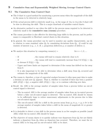
upSample 880.007503330.01477159SubgroupStd Dev0.0205 0.029400000.0193 0.031200000.0182 0.026000000.0171 0.023600000.0160 0.022000000.0149 0.022200000.0137 0.013000000.0126 0.014800000.0115 0.007400000.0104 0.006600000.0093 0.010000000.0082 0.004000000.0070 0.013800000.0059 0.015400000.0048 0.014000000.0037 0.019800000.0026 0.021800000.0014 0.017600000.0003 0.02080000-0.0008 0.02080000-0.0019 0.02520000-0.0030 0.02180000-0.0041 0.01880000-0.0053 06410.0652V-MaskUpperCusumLimit-0.0064 0.01020000V-MaskLowerLimitCumulative Sum Chart Summary for diameterThe CUSUM ProcedureCUSUM for Piston-Ring Diameters (sigma known) We will now make a cusum plot for the 25 sample means (n 5) assuming a process in-controlmean µ0 74 with process standard deviation σ .005 (known or specified prior to datacollection).CUSUM for Piston-Ring Diameters (sigma known)The CUSUM Procedure
ecisionDecision IntervalCusum Interval ubgroupSample 880.007503330.01477159SubgroupStd perUpperUpperUpperDecisionDecision IntervalCusum Interval ExceededCumulative Sum Chart Summary for diameterCumulative Sum Chart Summary for diameterSubgroupStd DevThe CUSUM ProcedureThe CUSUM ProcedureSubgroupSample SubgroupsampleSizeMeanUPPER ONE-SIDED CUSUMLOWER ONE-SIDED CUSUM We will now generate the upper and lower tabular cusums for the 25 sample meansfollowed by one-sided cusum plots.
UPPER ONE-SIDED CUSUMThe CUSUM ProcedureLOWER ONE-SIDED CUSUMThe CUSUM Procedure172
SAS Cusum Code for Piston-Ring Diameter DataDM ’LOG; CLEAR; OUT; CLEAR;’;OPTIONS NODATE NONUMBER;DATA piston;DO sample 1 TO 25;DO item 1 TO 5;INPUT diameter @@;diameter diameter 70; OUTPUT;END; END;LINES;4.030 4.002 4.019 3.992 4.0083.995 3.992 4.001 4.011 4.0043.988 4.024 4.021 4.005 4.0024.002 3.996 3.993 4.015 4.0093.992 4.007 4.015 3.989 4.0144.009 3.994 3.997 3.985 3.9933.995 4.006 3.994 4.000 4.0053.985 4.003 3.993 4.015 3.9884.008 3.995 4.009 4.005 4.0043.998 4.000 3.990 4.007 3.9953.994 3.998 3.994 3.995 3.9904.004 4.000 4.007 4.000 3.9963.983 4.002 3.998 3.997 4.0124.006 3.967 3.994 4.000 3.9844.012 4.014 3.998 3.999 4.0074.000 3.984 4.005 3.998 3.9963.994 4.012 3.986 4.005 4.0074.006 4.010 4.018 4.003 4.0003.984 4.002 4.003 4.005 3.9974.000 4.010 4.013 4.020 4.0033.988 4.001 4.009 4.005 3.9964.004 3.999 3.990 4.006 4.0094.010 3.989 3.990 4.009 4.0144.015 4.008 3.993 4.000 4.0103.982 3.984 3.995 4.017 4.013;SYMBOL1 v dot width 3;PROC CUSUM DATA piston;XCHART diameter*sample ’1’/ MU0 74 SIGMA0 .005 H 4.0 K 0.5 DELTA 1.0DATAUNITS HAXIS 1 TO 25TABLESUMMARY OUTTABLE qsum ;INSET ARL0 ARLDELTA H K SHIFT / POS n;LABEL diameter ’Diameter Cusum’sample ’Piston Ring Sample’;TITLE ’CUSUM for Piston-Ring Diameters (sigma known)’;PROC CUSUM DATA piston;XCHART diameter*sample ’1’/ MU0 74 SIGMA0 .005 H 4.0 K 0.5 DELTA 1.0DATAUNITS HAXIS 1 TO 25SCHEME onesided TABLESUMMARY TABLEOUT;INSET ARL0 ARLDELTA H K SHIFT / POS n;LABEL diameter ’Diameter Cusum’sample ’Piston Ring Sample’;TITLE ’UPPER ONE-SIDED CUSUM’;173
PROC CUSUM DATA piston;XCHART diameter*sample ’1’/ MU0 74 SIGMA0 .005 H 4.0 K 0.5 DELTA -1.0DATAUNITS HAXIS 1 TO 25SCHEME onesided TABLESUMMARY TABLEOUT;INSET ARL0 H K SHIFT / POS ne;LABEL diameter ’Diameter Cusum’sample ’Piston Ring Sample’;TITLE ’LOWER ONE-SIDED CUSUM’;*** The following code will make a table with resetting ***;***after an out-of-control signal is detected***;DATA qsum; SET qsum;h 4;k .5;sigma .005;aim 74;** enter values **;xbar subx ; n subn ;hsigma h*sigma/SQRT( subn );ksigma k*sigma/SQRT( subn );RETAIN cusum l 0 cusum h 0;IF (-hsigma cusum l hsigma)THEN DO;cusum l cusum l (aim - ksigma) - xbar;IF cusum l 0 then cusum l 0;END;IF (-hsigma cusum h hsigma)THEN DO;cusum h cusum h xbar - (aim ksigma);IF cusum h 0 then cusum h 0;END;IF MAX(cusum l,cusum h) ge hsigmaTHEN DO;IF (cusum l ge hsigma) THEN DO;flag ’lower’; OUTPUT; END;IF (cusum h ge hsigma) THEN DO;flag ’upper’; OUTPUT; END;cusum l 0; cusum h 0;END;ELSE OUTPUT;PROC PRINT DATA qsum;ID sample;VAR xbar n cusum l hsigma cusum h flag;TITLE ’CUSUM with Reset after Signal (sigma known)’;RUN;174
9 Cumulative Sum and Exponentially Weighted Moving Average Control Charts 9.1 The Cumulative Sum Control Chart The x-chart is a good method for monitoring a process mean when the magnitude of the shift in the mean to be detected is relatively large. If the actual process shift is relatively small (e.g., in the range of :5 x to 1 x),the x-chart will be slow in detecting the shift.