Transcription
PrimerBayesian statistics and modellingRens van de Schoot1 , Sarah Depaoli2, Ruth King3,4, Bianca Kramer5, Kaspar Märtens6,Mahlet G. Tadesse7, Marina Vannucci8, Andrew Gelman9, Duco Veen1, Joukje Willemsen1and Christopher Yau4,10Abstract Bayesian statistics is an approach to data analysis based on Bayes’ theorem, whereavailable knowledge about parameters in a statistical model is updated with the information inobserved data. The background knowledge is expressed as a prior distribution, and combinedwith observational data in the form of a likelihood function to determine the posteriordistribution. The posterior can also be used for making predictions about future events. ThisPrimer describes the stages involved in Bayesian analysis, from specifying the prior and datamodels to deriving inference, model checking and refinement. We discuss the importance ofprior and posterior predictive checking, selecting a proper technique for sampling from aposterior distribution, variational inference and variable selection. Examples of successfulapplications of Bayesian analysis across various research fields are provided, including in socialsciences, ecology, genetics, medicine and more. We propose strategies for reproducibility andreporting standards, outlining an updated WAMBS (when to Worry and how to Avoid the Misuseof Bayesian Statistics) checklist. Finally, we outline the impact of Bayesian analysis on artificialintelligence, a major goal in the next decade.Prior distributionBeliefs held by researchersabout the parameters in astatistical model before seeingthe data, expressed asprobability distributions.Likelihood functionThe conditional probabilitydistribution of the givenparameters of the data,defined up to a constant.Posterior distributionA way to summarize one’supdated knowledge, balancingprior knowledge with observeddata.Bayesian statistics is an approach to data analysis andparameter estimation based on Bayes’ theorem. Uniquefor Bayesian statistics is that all observed and unobserved parameters in a statistical model are given ajoint probability distribution, termed the prior and datadistributions. The typical Bayesian workflow consistsof three main steps (Fig. 1): capturing available knowledge about a given parameter in a statistical model viathe prior distribution, which is typically determined beforedata collection; determining the likelihood function usingthe information about the parameters available in theobserved data; and combining both the prior distribution and the likelihood function using Bayes’ theorem inthe form of the posterior distribution. The posterior distribution reflects one’s updated knowledge, balancing priorknowledge with observed data, and is used to conductinferences. Bayesian inferences are optimal when averaged over this joint probability distribution and inference for these quantities is based on their conditionaldistribution given the observed data.The basis of Bayesian statistics was first described in a1763 essay written by Reverend Thomas Bayes and published by Richard Price1 on inverse probability, or how todetermine the probability of a future event solely basedon past events. It was not until 1825 that Pierre SimonLaplace2 published the theorem we now know as Bayes’theorem (Box 1). Although the ideas of inverse probability and Bayes’ theorem are longstanding in mathematics, Q2Q3Q4 e- mail: 586-020-00001-2 Nature Reviews Methods Primersthese tools became prominent in applied statistics in thepast 50 years3–10. We will describe many advantages anddisadvantages throughout the Primer.This Primer provides an overview of the currentand future use of Bayesian statistics that is suitable forquantitative researchers working across a broad rangeof science- related areas that have at least some knowledge of regression modelling. We supply an overviewof the literature that can be used for further study andillustrate how to implement a Bayesian model on realdata. All of the data and code are available for teachingpurposes. This Primer discusses the general frameworkof Bayesian statistics and introduces a Bayesian researchcycle (Fig. 1). We first discuss formalizing of prior distributions, prior predictive checking and determiningthe likelihood distribution (Experimentation). We discuss relevant algorithms and model fitting, describeexamples of variable selection and variational inference, and provide an example calculation with posterior predictive checking (Results). Then, we describehow Bayesian statistics are being used in different fieldsof science (Applications), followed by guidelines fordata sharing, reproducibility and reporting standards(Reproducibility and data deposition). We concludewith a discussion on avoiding bias introduced by usingincorrect models (Limitations and optimizations), andprovide a look into the future with Bayesian artificialintelligence (Outlook).10123456789();
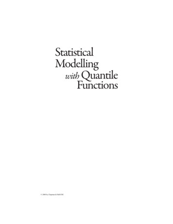
PrimerInformativenessPriors can have different levelsof informativeness and can beanywhere on a continuum fromcomplete uncertainty torelative certainty, but wedistinguish between diffuse,weakly and informative priors.HyperparametersParameters that define theprior distribution, such asmean and variance for anormal prior.Prior elicitationThe process by whichbackground information istranslated into a suitable priordistribution.Q5ExperimentationThis section outlines the first two steps in the Bayesianworkflow described in Fig. 1. Prior distributions, shortened to priors, are first determined. The selection ofpriors is often viewed as one of the more importantchoices that a researcher makes when implementing aBayesian model as it can have a substantial impact onthe final results. The appropriateness of the priors beingimplemented is ascertained using the prior predictivechecking process. The likelihood function, shortened tolikelihood, is then determined. The likelihood is combined with the prior to form the posterior distribution,or posterior (Results). Given the important roles that theprior and the likelihood have in determining the posterior, it is imperative that these steps be conducted withcare. We provide example calculations throughout todemonstrate the process.Empirical example 1: predicting PhD delaysTo illustrate many aspects of Bayesian statistics we provide an example based on real- life data. Consider anempirical example of a study predicting PhD delays11in which the researchers asked 333 PhD recipients inThe Netherlands how long it had taken them to complete their doctoral thesis. Based on this information,the researchers computed the delay — defined as the difference between the planned and the actual project timein months (mean 9.97, minimum/maximum –31/91,standard deviation 14.43). Suppose we are interested inpredicting PhD delay (y) using a simple regression model,y βintercept βage β age2 ε, with βage representing thelinear effect of age (in years). We expect this relation tobe quadratic, denoted by β age2. The model contains anintercept, βintercept, and we assume the residuals, ε, are normally distributed with mean zero and with an unknownvariance, σε2. Note that we have simplified the statisticalmodel, and so the results are only meant for instructionalpurposes. Instructions for running the code are availablefor different software12, including steps for data exploration13. We will refer to this example throughout thefollowing sections to illustrate key concepts. Formalizing prior distributionsPrior distributions play a defining role in Bayesian statistics. Priors can come in many different distributionalforms, such as a normal, uniform or Poisson distribution, among others. Priors can have different levelsof informativeness; the information reflected in a priorAuthor addressesDepartment of Methods and Statistics, Utrecht University, Utrecht, The Netherlands.Department of Quantitative Psychology, University of California Merced, Merced,CA, USA.3School of Mathematics, University of Edinburgh, Edinburgh, UK.4The Alan Turing Institute, British Library, London, UK.5Utrecht University Library, Utrecht University, Utrecht, The Netherlands.6Department of Statistics, University of Oxford, Oxford, UK.7Department of Mathematics and Statistics, Georgetown University, Washington, DC, USA.8Department of Statistics, Rice University, Houston, TX, USA.9Department of Statistics, Columbia University, New York, NY, USA.10Division of Informatics, Imaging & Data Sciences, University of Manchester,Manchester, UK.122 Article citation ID: #####################distribution can be anywhere on a continuum from complete uncertainty to relative certainty. Although priorscan fall anywhere along this continuum, there are threemain classifications of priors that are used in the literature to categorize the degree of (un)certainty surrounding the population parameter value: informative, weaklyinformative and diffuse. These classifications can bemade based on the researcher’s personal judgement. Forexample, a normal distribution is defined by a mean anda variance, and the variance (or width) of the distributionis linked to the level of informativeness. A variance of1,000 may be considered diffuse in one research settingand informative in another, depending on the values ofthe parameter as well as the scaling for the parameter.The relationship between the likelihood, prior andposterior for different prior settings for βage from ourexample calculation predicting PhD delays is shown inFig. 2. The first column represents the prior, which hasa normal distribution for the sake of this example. Thefive different rows of priors represent the different priorsettings based on the level of informativeness and variance from the mean. The likelihood, based on the data,is represented by a single distribution. The prior and thelikelihood are combined together to create the posterior according to Bayes’ rule. The resulting posterior isdependent on the informativeness (or variance) of theprior, as well as the observed data. We demonstrate howto obtain the posterior in the Results section.The individual parameters that control the amountof uncertainty in the priors are called hyperparameters.Take a normal prior as an example. This distribution isdefined by a mean and a variance that are the hyperparameters for the normal prior, and we can write this distribution as N μ0, σ02 , where μ0 represents the mean andσ02 represents the variance. A larger variance representsa greater amount of uncertainty surrounding the mean,and vice versa. For example, Fig. 2 illustrates five priorsettings with different values for μ0 and σ02. The diffuseand weakly informative priors show more spread thanthe informative priors, owing to their larger variances.The mean hyperparameter can be seen as the peak inthe distribution.()Prior elicitation. Prior elicitation is the process by whicha suitable prior distribution is constructed. Strategiesfor prior elicitation include asking an expert or a panelof experts to provide values for the hyperparameters ofthe prior distribution14–17. MATCH18 is a generic expertelicitation tool, but many methods that can be used toelicit information from experts require custom elicitation procedures and tools. For examples of elicitationprocedures designed for specific models, see refs19–23.For an abundance of elicitation examples and methods,we refer the reader to the TU Delft expert judgementdatabase of more than 67,000 elicited judgements24 (seealso14,25,26). Also, the results of a previous publication ormeta- analysis can be used27,28, or any combination29 orvariation of such strategies.Prior elicitation can also involve implementing databased priors. Then, the hyperparameters for the priorare derived from the sample data using methods suchas maximum likelihood30–33 or sample statistics34–36.www.nature.com/NRMP0123456789();
PrimerbSearch for background knowledgeP( )PriorPrior predictivecheckingPriorelicitationFormalizing priordistributionsaLiterature and theoryDefineproblemSpecifyhypothesisSearch for background knowledgeP(y )LikelihoodResearchquestionCollect data andcheck assumptionsPreprocessand clean dataSpecify analytic strategyDesign datacollectionstrategyDeterminelikelihood functionSelectmodel typeImplement samplingmethodP(y )PosteriorCompute posteriordistributionsModel specificationand variable selectionPosterior lysisComputeBayes factorsPosterior inferenceFig. 1 The Bayesian research cycle. The steps needed for a research cycle using Bayesian statistics include those of astandard research cycle and a Bayesian- specific workflow. a Standard research cycle involves reading literature, defininga problem and specifying the research question and hypothesis249,250. The analytic strategy can be pre- registered to enhancetransparency. b Bayesian- specific workflow includes formalizing prior distributions based on background knowledgeand prior elicitation, determining the likelihood function by specifying a data- generating model and including observeddata, and obtaining the posterior distribution as a function of both the specified prior and the likelihood function134,251.After obtainingthe posterior results, inferences can be made that can then be used to start a new research cycle. θ, fixed parameters; P, conditional probability distribution; y, data.Q1Informative priorA reflection of a high degreeof certainty or knowledgesurrounding the populationparameters. Hyperparametersare specified to expressparticular informationreflecting a greater degree ofcertainty about the modelparameters being estimated.These procedures lead to double- dipping, as the samesample data set is used to derive prior distributionsand to obtain the posterior. Although databased priorsare relatively common, we do not recommend the useof double- dipping procedures. Instead, a hierarchicalmodelling strategy can be implemented, where priorsdepend on hyperparameter values that are data- driven— for example, sample statistics pulled from the sample data — which avoids the direct problems linked todouble- dipping. We refer the reader elsewhere34 for moredetails on double- dipping.Prior (un)certainty. An informative prior is one thatreflects a high degree of certainty about the modelparameters being estimated. For example, an informativeNature Reviews Methods Primersnormal prior would be expected to have a very small variance. A researcher may want to use an informative priorwhen existing information suggests restrictions on thepossible range of a particular parameter, or a relationshipbetween parameters, such as a positive but imperfectrelationship between susceptibility to various medicalconditions37,38. In some cases, an informative prior canproduce a posterior that is not reflective of the population model parameter. There are circumstances wheninformative priors are needed, but it is also importantto assess the impact these priors have on the posteriorthrough a sensitivity analysis as discussed below. Anarbitrary example of an informative prior for our empirical example is βage N(2.5, 5), with a prior mean for thelinear relation of age with PhD delay of 2.5 and a prior30123456789();
PrimerBox 1 Bayes’ theoremRényi’s axiom of probability254 lends itself to examining conditional probabilities, wherethe probabilities of Event A and Event B occurring are dependent, or conditional. Thebasic conditional probability can be written as:p(B A) p(B A),p(A)(1)where the probability p of Event B occurring is conditional on Event A. Equation 1 setsthe foundation for Bayes’ rule, which is a mathematical expression of Bayes’ theoremthat recognizes p(B A) p(A B) but p(B A) p(A B), where the notation represents anintersection — or joint probability. Bayes’ rule can be written as:p(A B) p(A B),p(B)(2)which, based on Eq. 1, can be reworked as:p(A B) p(B A)p(A).p(B)(3)Equation 3 is Bayes’ rule. These principles can be extended to the situation of dataand model parameters. With data set y and model parameters θ, Eq. 3 (Bayes’ rule) canbe written as follows:p(θ y ) p(y θ )p(θ ),p(y )(4)which is often simplified to:p(θ y ) p(y θ )p(θ ).(5)The term p(θ y) represents a conditional probability, where the probability ofthe model parameters (θ) is computed conditional on the data (y), representing theposterior distribution. The term p(y θ) represents the conditional probabilityof the data given the model parameters, and this term represents the likelihoodfunction. Finally, the term p(θ) represents the probability of particular modelparameter values existing in the population, also known as the prior distribution.The term p(y) is often viewed as a normalizing factor across all outcomes y, whichcan be removed from the equation because θ does not depend on y or p(y). Theposterior distribution is proportional to the likelihood function multiplied bythe prior distribution.Weakly informative priorA prior incorporating someinformation about thepopulation parameter butthat is less certain thanan informative prior.Diffuse priorsReflections of completeuncertainty about populationparameters.Improper priorsPrior density functions that aredefined based on the data ordo not integrate to one, andas such are not a properdistribution but can generatea valid posterior distribution.variance of 5. A ShinyApp was developed specificallyfor the PhD example containing a visualization of howthe different priors for all parameters in the regressionmodel interact39.A weakly informative prior has a middling amount ofcertainty, being neither too diffuse nor too restrictive.A weakly informative normal prior would have a largervariance hyperparameter than an informative prior.Such priors will have a relatively smaller impact on theposterior compared with an informative prior, depending on the scale of the variables, and the posterior resultsare weighted more by the data observations as expressedin the likelihood.A researcher may want to use a weakly informativeprior when some information is assumed about a parameter, but there is still a desired degree of uncertainty. InFig. 2, the two examples of weakly informative normalpriors for the regression coefficient could allow 95%of the prior density mass to fall within values between4 Article citation ID: #####################–10 and 10 or between 0 and 10. Weakly informativepriors supply more information than diffuse priors, butthey typically do not represent specific information likean informative prior40,41. When constructing a weaklyinformative prior, it is typical to specify a plausibleparameter space, which captures a range of plausibleparameter values — those within a reasonable rangeof values for the select parameter (for an example, seethe ShinyApp we developed for the PhD example39)— and excludes improbable values by attaining only alimited density mass at implausible values. For example,if a regression coefficient is known to be near 0, thena weakly informative prior can be specified to reducethe plausible range to, for example, 5. This prior wouldreduce the probability of observing out- of- bound values (for example, a regression coefficient of 100) withoutbeing too informative.Finally, a diffuse prior reflects a great deal of uncertainty about the model parameter. This prior formrepresents a relatively flat density and does not includespecific knowledge of the parameter (Fig. 2). A researchermay want to use a diffuse prior when there is a completelack of certainty surrounding the parameter. In this case,the data will largely determine the posterior. Sometimes,researchers will use the term non- informative prior as asynonym for diffuse42. We refrain from using this termbecause we argue that even a completely flat prior, suchas the Jeffreys prior43, still provides information aboutthe degree of uncertainty44. Therefore, no prior is trulynon- informative.Diffuse priors can be useful for expressing a complete lack of certainty surrounding parameters, but theycan also have unintended consequences on the posterior45. For example, diffuse priors can have an adverseimpact on parameter estimates via the posterior whensample sizes are small, especially in complex modellingsituations involving meta- analytic models46, logisticregression models44 or mixture models47. In addition,improper priors are sometimes used with the intention ofusing them as diffuse priors. Although improper priorsare common and can be implemented with relative easewithin various Bayesian programs, it is important to notethat improper priors can lead to improper posteriors. Wemention this caveat here because obtaining an improperposterior can impact the degree to which results can besubstantively interpreted. Overall, we note that a diffuseprior can be used as a placeholder before analyses ofthe same or subsequent data are conducted with moreinformative priors.Impact of priors. Overall, there is no right or wrongprior setting. Many times, diffuse priors can produceresults that are aligned with the likelihood, whereassometimes inaccurate or biased results can be obtainedwith relatively flat priors47. Likewise, an informativeprior that does not overlap well with the likelihood canshift the posterior away from the likelihood, indicating that inferences will be aligned more with the priorthan the likelihood. Regardless of the informativenessof the prior, it is always important to conduct a priorsensitivity analysis to fully understand the influencethat the prior settings have on posterior estimates48,49.www.nature.com/NRMP0123456789();
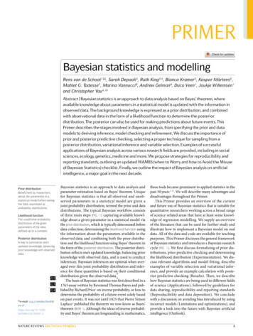
PrimerWhen the sample size is small, Bayesian estimationwith mildly informative priors is often used9,50,51, butthe prior specification might have a huge effect on theposterior results.When priors do not conform with the likelihood, thisis not necessarily evidence that the prior is not appropriate. It may be that the likelihood is at fault owing toa mis- specified model or biased data. The differencebetween the prior and the likelihood may also be reflective of variation that is not captured by the prior orlikelihood alone. These issues can be identified througha sensitivity analysis of the likelihood, by examiningP( )Priordifferent forms of the model, for example, to assess howthe priors and the likelihood align.The subjectivity of priors is highlighted by critics as apotential drawback of Bayesian methods. We argue twodistinct points here. First, many elements of the estimation process are subjective, aside from prior selection,including the model itself and the error assumptions.To place the notion of subjectivity solely on the priorsis a misleading distraction from the other elements inthe process that are inherently subjective. Second, priorsare not necessarily a point of subjectivity. They can beused as tools to allow for data- informed shrinkage, enactP( y)PosteriorP(y )LikelihoodDiffuse0.40.400 –10010βage Weakly informative0.40.40–100βage N(0,25)010Weakly informative0.40.40.4 0 –1000 –1010βage N(6,25)Informative–101000.40.4000010βage N(2.5,5)Informative110–100010βage N(2.5,0.2)Fig. 2 Illustration of the key components of Bayes’ theorem. The prior distribution (blue) and the likelihood function(yellow) are combined in Bayes’ theorem to obtain the posterior distribution (green) in our calculation of PhD delays.Five example priors are provided: one diffuse, two weakly informative with different means but the same variance andtwo informative with the same mean but different variances. The likelihood remains constant as it is determined bythe observed data. The posterior distribution is a compromise between the prior and the likelihood. In this example, theposterior distribution is most strongly affected by the type of prior: diffuse, weakly informative or informative. βage, lineareffect of age (years); θ, fixed parameters; P, conditional probability distribution; y, data.Nature Reviews Methods Primers50123456789();
Primerpriors. The majority of the discussion in this Primerpertains to univariate priors placed on individual modelparameters; however, these concepts can be extended tothe multivariate sense, where priors are placed on anentire covariance matrix rather than a single elementfrom a matrix, for example. For more information onmultivariate priors, see refs52,53.Box 2 Bayes factorsHypothesis testing consists of using data to evaluate the evidence for competingclaims or hypotheses. In the Bayesian framework, this can be accomplished usingthe Bayes factor, which is the ratio of the posterior odds to the prior odds of distincthypotheses43,64. For two hypotheses, H0 and H1, and observed data y, the Bayes factorin favour of H1, denoted BF10, is given by:BF10 p(H1 y ) / p(H0 y ),p(H1) / p(H0)(6)where the prior probabilities are p(H0) and p(H1) 1 – p(H0). A larger value of BF10 providesstronger evidence against H0 (ref.64). The posterior probability of hypothesis Hj, p(Hj y),for j 0 or 1, is obtained using Bayes theorem:( )p Hj y p(y Hj)p(Hj)p(y ).(7)Thus, the Bayes factor can equivalently be written as the ratio of the marginallikelihoods of the observed data under the two hypotheses:BF10 p(y H1).p(y H0)(8)The competing hypotheses can take various forms and could be, for example, twonon- nested regression models. If H0 and H1 are simple hypotheses in which theparameters are fixed (for example, H0: μ μ0 versus H1: μ μ1), the Bayes factor isidentical to the likelihood ratio test. When either or both hypotheses are composite orthere are additional unknown parameters, the marginal likelihood p(y Hj) is obtained byintegrating over the parameters θj with prior densities p(θj Hj). This integral is oftenintractable and must be computed by numerical methods. If p(θj Hj) is improper (forexample, p θj Hj dθj ), then p(y Hj) will be improper and the Bayes factor will not beuniquely defined. Overly diffuse priors should also be avoided, as they result in a Bayesfactor that favours H0 regardless of the information in the data104.As a simple illustrative example, suppose one collects n random samplesfrom a normally distributed population with an unknown mean μ and a knownvariance σ2, and wishes to test H0: μ μ0 versus H1: μ μ0. Let y be the samplemean. H0 is a simple hypothesis with a point mass at μ0, so y H0 N(µ0, σ 2/n).Under H1, y µ, H1 N(µ, σ 2/n) and assuming μ H1 N(μ0, τ2) with τ2 fixed, thenp(y H1) p(y µ, H1)p(µ H1)dµ reduces to y H1 N(µ0, τ 2 σ 2/n). Thus, the Bayesfactor in favour of H1 is:( ) (y µ 0 )2 exp 2 2 2(τ σ /n ) (y µ 0 )2 1/22 (σ /n) exp 2 2 σ /n ( ) 1/2BF10 p(y H1) p(y H0)22(τ σ /n)(10)For example, for n 20, y 5.8, μ0 5, σ2 1 and τ2 1, the Bayes factor is BF10 96.83,which provides strong evidence that the mean μ is not 5.Prior predictive checkingThe process of checkingwhether the priors make senseby generating data accordingto the prior in order to assesswhether the results are withinthe plausible parameter space.Prior predictive distributionAll possible samples that couldoccur if the model is truebased on the priors.regularization or influence algorithms towards a likelyhigh- density region and improve estimation efficiency.Priors are typically defined through previous beliefs,information or knowledge. Although beliefs can be characterized as subjective points of view from the researcher,information is typically quantifiable, and knowledge canbe defined as objective and consensus- based. Therefore,we urge the reader to consider priors in this broadersense, and not simply as a means of incorporatingsubjectivity into the estimation process.This section on informative, weakly informative anddiffuse priors was written in a general sense, with theseterms applicable to both univariate and multivariate6 Article citation ID: #####################Prior predictive checkingBecause inference based on a Bayesian analysis issubject to the ‘correctness’ of the prior, it is of importance to carefully check whether the specified modelcan be considered to be generating the actual data54,55.This is partly done by means of a process known asprior predictive checking. Priors are based on backgroundknowledge and cannot be inherently wrong if the priorelicitation procedure is valid, that is, if the backgroundknowledge is correctly expressed in probability statements. However, even in the case of a valid prior elicitation procedure, it is extremely important to understandthe exact probabilistic specification of the priors. This isespecially true for complex models with smaller samplesizes9. Because smaller sample sizes usually convey lessinformation, priors, in comparison, will exhibit a stronginfluence on the posteriors. Prior predictive checking isan exercise to improve the understanding of the implications of the specified priors on possible observations.It is not a method for changing the original prior, unlessthis prior explicitly generates incorrect data.Box56 suggested deriving a prior predictive distributionfrom the specified prior. The prior predictive distribution is a distribution of all possible samples that couldoccur if the model is true. In theory, a ‘correct’ priorprovides a prior predictive distribution similar to thetrue data- generating distribution54. Prior predictivechecking compares the observed data, or statistics of theobserved data, with the prior predictive distribution, orstatistics of the predictive distribution, and checks theircompatibility55. For instance, values are drawn from theprior distributions. Using kernel density estimation, anon- parametric smoothing approach used to approximate a probability density function57, the original sampleand the samples from the predictive distribution can becompared58. Alternatively, the compatibility can summarized by a prior predictive p- value, describing how farthe characteristics of the observed da
edge of regression modelling. We supply an overview of the literature that can be used for further study and illustrate how to implement a Bayesian model on real data. All of the data and code are available for teaching purposes. This Primer discusses the general framework of Bayesian statis