WIXLIB

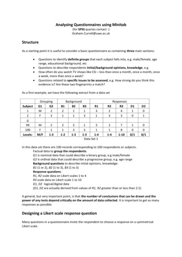
Analysing Questionnaires using Minitab(for SPSS queries contact -)Graham.Currell@uwe.ac.ukStructureAs a starting point it is useful to consider a basic questionnaire as containing three main sections: Questions to identify definite groups that each subject falls into, e.g. male/female, agerange, educational background, etcQuestions to describe respondents initial/background opinions, knowledge, e.g.How often do you watch TV shows like CSI – less than once a month, once a month, oncea week, more than once a week?Questions related to specific issues to be assessed, e.g. How strong do you think thisevidence is? Are these two fingerprints a match?As a first example, we have the following extract from a data setSubject12 B2B3211113211-2331-3R13113311-31-4Data Set 1ResponsesR2R32433D110D201211-4100/1000/1781-10In this data set there are 100 records corresponding to 100 respondents or subjects.Factual data to group the respondents:G1 is nominal data that could describe a binary group, e.g male/femaleG2 is ordinal data that could describe a progressive group, e.g. age rangeBackground questions to describe initial opinions, knowledge:B1 (1 or 2), B2 (1 to 3), B3 (1 to 3)Response questions:R1, R2 scale data on Likert scales 1 to 4R3 scale data on Likert scale 1 to 10D1, D2 logical/digital data(D1, D2 are actually derived from values of R1, R2 greater than or less than 2.5)A general, but very important point, is that the number of conclusions that can be drawn and thepower of any tests depend critically on the amount of data collected. It is important to get as manyresponses as possible.Designing a Likert scale response questionMany questions in a questionnaire invite the respondent to choose a response on a symmetricalLikert scale.

For example:Do you agree with a particular a statement? Give your answer on thescale between Disagree strongly is -3 to Agree strongly is 3:-3 -2 -1 0 1 2 3or betweenDisagree strongly is 1 to Agree strongly is 4:1 2 3 4(it does not make any difference to the analysis if you code answers 1 to 7 instead of -3 to 3)One factor to consider is whether you wish to have a neutral, ‘0’, answer (neither agree or disagree)or whether you force the respondent to choose ‘-‘ or ‘ ’. This might depend on the question.Forcing ‘-‘ or ‘ ’ could give you a binary answer with the option of using simple, yes/no, proportions,but is it ‘right’ to deny the neutral option?It is also important to consider how many levels you should include in your scale.If you have too few, then you might find that almost all of the respondents give the same answer,e.g. on a scale of 1 to 4, everyone might reply ‘3’, making it impossible to do detailed analysis.If you have too many, then using the frequency of responses in each category can become too smallfor useful analysis, e.g. in using chi-squared.Ideally a pilot study would reveal the ranges of answers that could be expected in a finalquestionnaire, allowing you to design the questions more sensitively, but this is not possible for yoursimple project.An alternative option is to use a larger number of levels, e.g. 1 to 9 and anticipate combining levels,depending on the responses obtained, see the 69 responses below:Original levels:Counts:-41-32-21-1409 122 219 38 43New levels:-10 1 2 3Counts:89221911Note that the above data reduction procedure should only be used for chi-squared frequencyanalysis.Useful analytical techniquesAt a basic level we could record the basic statistics of the data in each column, e.g.The mean response to R3 was 4.13 with a standard deviation of 0.22The proportion of ‘1’ responses to D1 was 0.64The proportion of ‘1’ responses to D2 was 0.60This might tell us the how subjects, in general, responded to each question, but it would not give anyinformation about any relationships hidden within the data, e.g.Does the mean response to R3 differ for different G2 groups?Do the subjects who respond ‘1’ for D1 also respond ‘1’ for D2?In the following sections we look at various techniques that you might find useful.

1. Using boxplots to explore raw dataBoxplots are an excellent way to explore yourown data and to present raw data in your report.Boxplot of R31086R3In the example, the boxplot of response R3,grouped separately for M and F responses to G1,suggests that there is no difference in themedian value, but is there a difference in thespread or variance?Is the outlier significant?420FMG12. Using histograms to check data distributionsSometimes you may see a bi-modal responsewith two different groups giving two differentresponses with two clear peaks.Histogram of R32015FrequencyA histogram can be useful when you haveseveral possible response levels to a question. Itshows how the replies are distributed.The example here shows a uni-modal response,with one main peak.10500246810R33. Is there a difference in the average responses, R1, R2, R3 for the two values each of G1, B1?Using t-test R1 and R3 shows significant differences in the mean responses for the two B1 groupswith p 0.009 and p 0.004 respectively.Mann-Whitney is preferable for data without normal distribution (Minitab needs data in twocolumns) giving p 0.003 and p 0.010 for the same tests as the t-tests above.4. Is there a difference in the average responses R1, R2, R3 for the three values each of G2, B2, B3etc ?Using One-Way ANOVA to test whether the mean of R1 changes for different values of 00.9661.046F4.47P0.014Individual 95% CIs For Mean Based onPooled StDev------- --------- --------- --------- *-----------)------- --------- --------- --------- -2.402.803.203.60Pooled StDev 1.099Mean of R1 is different for levels 1 and 2 from G2.Using Kruskal-Wallis also shows differences in R1 for different levels of G2, with p 0.017

5. Are there any interactions between possible factors, i.e. does one factor have a different effect,depending on the value of another factor?Using GLM to test whether R1 is affect by G2, B1 or an interaction between themAnalysis of Variance for R1, using AdjustedSource DFSeq SSAdj SS Adj MSFG2210.8006.5703.285 2.83B116.8838.0918.091 6.97G2*B121.2121.2120.606 0.52Error94 109.105 109.1051.161Total99 128.000SS for TestsP0.0640.0100.595These results give R1 dependent on B1 but not now significant for G2 (compare with 1-way ANOVAabove) and shows no significance for any interaction between them.Note: If you try to include too many factors or interactions, the available data is spread out andreduces the power of the individual analyses making a ‘not significant’ result more likely.6. Is there a difference in the variances of, R1, R2, R3 for the two values each of G1, B1?For example using the 2 variances test for R3 for the two groups in G1MethodF Test (normal)Levene's Test (any 1940.041which is not significant for the F-test, but Levene’s test suggests that there is a difference in thevariance of F responses compared to those of M (see boxplot in 1. above)7. Is there a difference in the proportion of ‘1’ responses between D1 and D2?Using the 2 proportions test:Fisher's exact test: P-Value 0.662There is no significant difference - see 9. below for the measure of agreement.8. Do the values of one answer change in the same way as those of another answer?For example: You might have good reason, from prior knowledge, to believe that the values of R1change in a similar way to the values of the respondents group B1.A test for correlation between R1 and B1 produces significant correlation with p 0.004However be aware that correlation is not the same as ‘cause and effect’.It is possible that B1 does not directly influence R1 (or vice versa), but both might be influenced by athird factor (see next example below).Alternatively, without any prior knowledge you might look randomly for any possible correlationsbetween all of the answer.A test for bivariate correlations between all of the answers gives:Correlations: G2, B1, B2, B3, R1, R2, R3G2B1B2B3-0.1560.121B2 -0.024 -0.0180.8130.862B30.048 -0.416 -0.0180.6380.0000.857R10.0940.2880.052 -0.3060.3500.0040.6070.002R20.0840.126 -0.003 -0.2390.4070.2110.9770.017R3 -0.1110.2610.275 -0.0950.2720.0090.0060.348Cell Contents: Pearson 668B1

In the above table the p-value is the lower value in the pair of values given for each combination ofvariables – check that the p-value for R1 and B1 is again given as 0.004.Bonferroni correction:You must be very careful with the above data because the chance of seeing a false significance (i.e. p 0.05 just by chance) has increased considerably because you have calculated many (n 21) pvalues.Where you are randomly looking for possible significant results amongst several p-values, theBonferroni correction gives a new 95% confidence critical value:Critical value 0.05/n where n is the number of p-values calculated.In this case the critical value would be 0.05/21 0.003B1 and B3, R1 and B3, R1 and R2 show significant correlation, but not R1 and B1!It is often possible that two variables might show correlation just because they are both correlatedwith the same third variable:e.g. R1 is correlated with B3 and B3 is correlated with B1, so it is likely that R1 and B1 show somecorrelation (see previous example above).SPSS can perform partial correlations where is possible to compensate for a third correlated variablewhen calculating the correlation between two variables.9. How good is the match, or agreement, between D1 and D2A test for correlation between D1 and D2 gives p 0.0005, but it is sometimes important to knowhow strong the agreement is between D1 and D2. For example, D1 and D2 might be twoassessments of the match of a fingerprint using different assessment protocols.Using Attribute Agreement Analysis for D1, D2Between AppraisersAssessment Agreement# Inspected # Matched10086Percent86.00Cohen's Kappa StatisticsResponseKappaSE Kappa00.703390 0.099640310.703390 0.099640395% CI(77.63, 92.13)Z7.059297.05929P(vs 0)0.00000.0000K 0.7 suggests a good matchThere is a variety of other measures available to measure of the strength of association betweenquestionnaire answers, which are grouped in the following table by the types of variables involved:nominal, ordinal and interval.They are also divided into two types: symmetrical and directional. In a directional (or asymmetric)association we measure how a knowledge of one (independent) variable can be used to predict thevariation of the other (dependent) variable. In a symmetric association, there is no sense of directionand we measure only the extent to which the two variables vary in similar ways.For further information on these statistics, contact Graham.Currell@uwe.ac.uk