WIXLIB

USING MINITAB: A SHORT GUIDE VIA EXAMPLESThe goal of this document is to provide you, the student in Math 112, with a guide to some of thetools of the statistical software package MINITAB as they directly pertain to the analysis of data you willcarry out in Math 112, in conjunction with the textbook Introduction to the Practice of Statistics by DavidMoore and George McCabe. This guide is organized around examples. To help you get started, it includespictures of some screens you'll see and printouts of the commands. It is neither a complete list ofMINITAB capabilities nor a complete guide to all of the uses of MINITAB with this textbook, but isdesigned to hit the highlights and a few sticking points, so to speak, of the use of MINITAB for problems inthe text, based on the Spring 1997 and Fall 1997 courses. For a brief dictionary of MINITAB functions andtheir EXCEL equivalents, plus more information about EXCEL, see elsewhere in this website. NOTE:This guide does update some of the MINITAB commands given in Introduction to the Practice of Statistics.CONTENTS1. Starting and running MINITAB on grounds2. Describing distributions (Ch. 1 of text)3. Scatterplots, Linear Regression, and Correlation (Ch. 2 of text)4. Inference for Regression (Section 10.1 of text)1. Starting and running MINITAB on grounds OPENING MINITABMINITAB should be available in any on-grounds computer lab. Begin from the Windows menu,and look for the folder marked STATISTICS ( or perhaps MATHEMATICS, if there is no STATISTICSfolder listed). Clicking to open this file, you should see the MINITAB icon (a blue- and white-stripedarrow, labelled MINITAB). Clicking on this will open MINITAB, displaying a 'session window' on top anda 'data window' below.

ENTERING DATAThe cursor can be placed in either window, but to begin to use MINITAB we will, of course, needto enter some data. Upon opening a new file, the data window should be ready to receive columns of data.Simply place the cursor in the first row (box) of column C1, enter the first number of your data set, and hit'Enter'. MINITAB will then automatically move down to the second row in this column, making data easyto enter. Note that you can label your column by entering a name in the box above the first row but stillbelow the label 'C1'. In order to have a data set to use when following the examples below, enter thefollowing numbers in C1:(*)56.65.26.17.4The data should appear in the data window as so:8.75.46.87.17.4

You can print out the data window at any time by locating your cursor anywhere inside thewindow, and clicking on the 'Print' icon below the toolbar. The printout will ignore empty columns. PRINTINGAs noted immediately above, the 'Print' icon (a little printer, of course) can be used to print out thedata window. Similarly, you can move the cursor to the session window to print the output placed in thiswindow by some of the commands we'll soon explore. You can also print graph windows by clicking on thegraph before attempting to print. GETTING HELP FROM MINITABThe 'Help' command in MINITAB is very useful. Once you have pulled up a command window,say by following some of the paths below ( see 'THE TOOLBAR AND COMMANDS' below ), you canclick on the HELP button to produce a description of the command and usually an accompanying example;these can be printed out using the 'Print' icon if you like. If you are trying to locate a feature, follow the'Search' option after clicking on the 'Help' command on the toolbar. You may want to use this to seek outmore information about the commands used below, or on topics not covered in this guide. When you beginthe course and do not yet have much knowledge of statistics, the information contained in the help sheets

can be a bit overwhelming, but with time and with some basic examples in your hands (as this guide hopesto help you acquire), negotiating MINITAB by using 'Help' becomes fairly easy. THE TOOLBAR AND COMMANDSThe tool bar on the top includes the and using the mouse to click on each of these produces a range of options. To indicate the path of acommand originating from the toolbar, we will use notation such asStat Basic Statistics Descriptive Statistics.Check that beginning with 'Stat' you can find the 'Basic Statistics' option, and from that the 'DescriptiveStatistics' selection as below:

A picture of the resulting command window is shown in the next section. (For now, hit the 'Cancel' buttonto close off the window without executing a command, as of yet!)Commands can be entered in the sessions window (or by pulling up a special window for enteringcommands), and in some places in the text, this is the way they suggest for you to use MINITAB. In thisguide we will instead, whenever possible, take advantage of the current format of MINITAB to 'mouse'along.2. Describing Distributions (Ch. 1 of text)NOTE: In the examples which follow, we will use the data set (*) from 'Entering Data' in Section 1of this guide above. This data will be referred to by the label 'C1'. For additional data sets, theseprocedures can be repeated by substituting their corresponding column labels in place of C1, or, inmost cases, the output can be produced for several different columns at the same time. We willdetail the procedure for a single column only. DESCRIPTIVE STATISTICS (MEAN, MEDIAN, QUARTILES, STANDARD DEVIATION.)For each column of data, you can find the mean, median, standard deviation, min, max, and firstand third quartiles all in one shot by following the command path Stat Basic Statistics DescriptiveStatistics and entering C1 in the 'Variables' box.

Graphs such as histograms and boxplots can be produced by selecting those options, or see those topicsseparately below. The output (without graphs) appears in the session window as shown below.Descriptive StatisticsVariableC1N10Mean6.570Median6.700Tr tDev1.163SE Mean0.368Many of these statistics (and some others such as the sum of squares and range) can also becomputed separately by following Calc Column Statistics and entering C1 as the 'Input variable'. HISTOGRAM

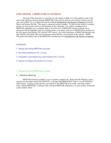
To produce a histogram of the data in C1, follow Graph Histogram. Enter C1 in the first rowunder 'Graph Variable' and click 'OK'. The output is a separate graph window as below. BOXPLOTUse Graph Boxplot and enter C1 in the first row of the 'Y' column under the 'Graph variables'heading, then click on 'OK'. The output appears in a graph window.

9C18765 STEMPLOT (STEM-AND-LEAF PLOT)Substitute C1 into the 'Variables' window appearing after following the path Graph CharacterGraph Stem-and-Leaf. The output appears in the session window.Character Stem-and-Leaf DisplayStem-and-leaf of C1Leaf Unit 0.10334(2)411155667788N 100241681447You might note that other graphs, such as histograms and boxplots, can also be created as character graphs,but they just aren't as pretty! TIME SERIES PLOTThis plot will, using the preset features, produce a time series plot labelled on the x-axis by thenumbers 1, 2, 3,. placed at equally spaced intervals, and with dots connected. Check the help menu forchanging this labelling. Take the path Graph Time Series Plot and enter C1 in the first row of the 'Y'column under 'Graph variables', then click 'OK'.

9C18765Index12345678910To produce a time series plot which labels the points by their order of appearance and does notconnect the dots, use the path Graph Character Graphs Time Series Plot.Character Multiple Time Series PlotC1 8.75 7.50 6.25 5.00 6509824731 ----- ----- ----- ----- ----- 0246810NORMAL QUANTILE PLOTAs your text notes, a normal quantile plot is also called a 'normal probability plot.' To produce aplot which corresponds to the text's definition of a normal quantile plot in MINITAB, you can use the pathGraph Probability Plot with C1 as the variable and 'Normal' as the selection under 'Assumeddistribution'. Click on 'OK'. Along with some other data, the graph appears as below:

Normal Probability Plot for 0105134567891011DataYou'll notice that the output includes some curves which do not appear in the text's illustrations ofnormal quantile plots. To produce a simpler picture, without these curves, you can follow the book'ssuggestion and create one yourself. To do this, first enter the command NSCORES C1 C5 in the prompt inthe session window. (If you already have some data in the session window and cannot get a prompt toappear there, you can also enter this command by following the path Edit Command Line Editor.) Thisproduces a new column of data, C5. If the C5 column is already filled before you begin this process,choose another label in its place (say, if C2 or C10 is empty). Now, to get a picture just like the text's,enter the new command PLOT C5 * C1 as above, or follow Graph Plot and substitute C5 for 'Y' and C1for 'X' in the first row of 'Graph Variables'.C510-156789C1As a final note, MINITAB includes other commands for producing normal probability plots andvariations such as NORMPLOT and following the path Stat Basic Statistics Normality Test. Youmay wish to check with your instructor to see if some variation other than the two described above isdesired.3. Scatterplots, Linear Regression, and Correlation (Ch. 2 of text)Note: In the examples which follow, we will use the data from Example 2.11 of the text. In this case,the 'x-variable' data is recorded as 'student' in column C1 of the data sheet, and the 'y-variable' dataas 'math' in column C2. You should thus enter the following data into the data session window:

Note that you can clear out any previous entries in these two columns by highlighting the boxes usingthe mouse, and by following EDIT CLEAR CELLS. SCATTERPLOTFollow Graph Plot and in the first row under 'Graph variables' enter C2 in the column for 'Y'and C1 in the column for 'X'. Hit 'OK'. As the text suggests, you can also enter the command PLOT C2 *

C1 in the session window (or by following the path Edit Command Line Editor if you cannot get aprompt in the session window). The output, which appears in a graph window, is shown below.math7500700065004000 4100 4200 4300 4400 4500 4600 4700 4800 4900student LINEAR REGRESSION: LEAST-SQUARES REGRESSION LINE AND CORRELATIONCOEFFICIENTThere are many features of MINITAB's 'Regression' command which we will want to explore.Let's begin simply by finding the equation for the least-squares regression line of 'Y' (here, 'math') on 'X'(here, 'student'). Instead of following the test's suggestion to enter commands into the session window, wewill take the command path Stat Regression Regression to pull up the following window:

Entering C2 in the 'Response' box and C1 in the 'Predictors' box as above, and selecting 'OK' gives thefollowing output in the session window:Regression Analysis