Transcription
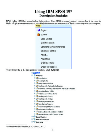
Using IBM SPSS 19*Descriptive StatisticsSPSS Help. SPSS has a good online help system. Once SPSS is up and running, you can find it by going toHelp Topics in the menu bar, i.e., click Help in the menu bar and then click Topics in the drop window that opens.You will now be in the help contents window. Click Tutorial.*Brother Walter Schreiner, FSC (July 1, 2011)1
You can then open any of the books comprising the tutorial by clicking on the to get to the various subtopics.Once in a subtopic is open, you can just keep clicking on the right and left arrows to move through it pageby page. I suggest going through the entire Overview booklet. Once you are working with a data set, and havean idea of what you want to do with the data, you can also use the Statistics Coach under the Help menu tohelp get the information you wish. It will lead you through the SPSS process.Using the SPSS Data Editor. When you begin SPSS, you open up to the Data Editor. For our purposes rightnow, you can learn how to do this by going to Help Tutorial Using the Data Editor, and then workingyour way through the subtopics. The data we will use is given in the table below, with the numbers indicatingtotal protein (μg/ml). .2459.3651.7061.9061.7079.5572.1066.6044.73For our data, double click on the var at the top of the first column or click on the Variable View tab at the bottom of the page, type in protein" in the Name column, and hit Enter. Under the assumption that you are goingto enter numerical data, the rest of the row is filled in.Changes in the type and display of the variable can be made by clicking in the appropriate cells and using anybuttons given. Then hit the Data View tab and type in the data values, following each by Enter.Save the file as usual where you wish under the name protein.sav. You just need type protein. The suffix isattached automatically.2
Sorting the Data. From the menu, choose Data Sort Cases , click the right arrow to move protein tothe Sort by box, make sure Ascending is chosen, and click OK. Our data column is now in ascending order.However, the first thing that come up is an output page telling you what has happened. Click the table with theStar on it to get back to the Data Editor.Obtaining the Descriptive Statistics. Go to Analyze Descriptive Statistics Explore.,select protein from the box on the left, and then click the arrow for Dependent List:. Make sure Both ischecked under Display.3
Click the Statistics. button, then make sure Descriptives and Percentiles are checked. We will use 95%for Confidence Interval for Mean. Click Continue.Then click Plots. Under Boxplots, select Factor levels together, and under Descriptive, choose bothStem-and-leaf and Histogram. Then click Continue.4
Then click OK. This opens an output window with two frames. The frame on the left contains an outline of thedata on the right.5
Clicking an item in either frame selects it, and allows you to copy it (and paste into a word processor), for instance. Double clicking an item in the left frame either shows or hides that item in the right frame. Clicking onDescriptives in the left frame brings up the following:The Standard Error of the Mean is a measure of how much the value of the mean may vary from repeatedsamples of the same size taken from the same distribution. The 95% Confidence Interval for Mean aretwo numbers that we would expect 95% of the means from repeated samples of the same size to fall between. The5% Trimmed Mean is the mean after the highest and lowest 2.5% of the values have been removed. Skewness measures the degree and direction of asymmetry. A symmetric distribution such as a normal distributionhas a skewness of 0, a distribution that is skewed to the left, when the mean is less than the median, has a negativeskewness, and a distribution that is skewed to the right, when the mean is greater than the median, has a positiveskewness. Kurtosis is a measure of the heaviness of the tails of a distribution. A normal distribution has kurtosis0. Extremely nonnormal distributions may have high positive or negative kurtosis values, while nearly normaldistributions will have kurtosis values close to 0. Kurtosis is positive if the tails are “heavier” than for a normaldistribution and negative if the tails are “lighter” than for a normal distribution.Double clicking an item in the right frame opens it's editor, if it has one. Double click on the histogram, shown onthe next page, to open the Chart Editor. To learn about the Chart Editor, visit Building Charts and Editing Charts under Help Core System. Once the chart editor opens, choose Edit Properties from theChart Editor Menus, click on a number on the vertical axis (which highlights all such numbers), and then click onScale. From the left diagram at the bottom of the next page, we see a minimum and a maximum for the verticalaxis and a major increment of 5. This corresponds to the tick marks and labels on the vertical axis. Now click onLabels & Ticks, check Display Ticks under Minor Ticks, and enter 5 for Number of minor ticks permajor ticks:. The Properties window should now look like the rightmost diagram at the bottom of the nextpage. Click Apply to see the results of this change.6
7
Now click on a number on the horizontal axis and then click on Number Format. In the diagram to the leftbelow, we see that we have 2 decimal places. The values in this window can be changed as desired. Next, clickon one of the bars and then Binning in the Properties window. Suppose we want bars of width 20 beginning at30. Check Custom, Interval width:, and enter 20 in the value box. Check Custom value for anchor:,followed by 30 in the value box. Your window should look like the one on the right below.Finally, click Apply and close the Chart Editor to get the histogram below.8
Next choose Percentiles from either output frame. The following comes up.Obviously, there are two different methods at work here. The formulas are given in the SPSS Algorithms Manual.Typically, use the Weighed Average. Tukey’s Hinges was designed by Tukey for use with the boxplot.The box covers the Interquartile range (IQR) Q75 - Q25, with the line being Q50, the median. In all three cases,the Tukey’s Hinges is used. The whiskers extend a maximum of 1.5 IQR from the box. Data points between1.5 and 3 IQR from the box are indicted by circles and are known as outliers, while those more than 3 IQR fromthe box are indicated by asterisks and are known as extremes. In this boxplot, the outliers are the 59th, 60th, and61st elements of the data list.Copying Output to Word (for instance). You can easily copy a selection of output or the entire output window to Word and other programs in the usual fashion. Just select what you wish to copy, choose Edit Copy,switch to a Word or other document and choose Edit Paste. After saving the output, you can also exportit as a Word, Powerpoint, Excel, text, or PDF document from File Export. For information on this, seeHelp Tutorial Working with Output or Help Core System Working with Output.Probability DistributionsBinomial Distribution. We shall assume n 15 and p .75. We will first find P(X x 15, .75) for x 0, ., 15,i.e., the cumulative probabilities. First put the numbers 0 through 15 in a column of a worksheet. (Actually, youonly need to enter the numbers whose cumulative probability you desire.) Then click Variable View, type innumber (the name you choose is optional) under Name, and I suggest putting in 0 for Decimal. Still in Variable View, put the names cum bin and bin prob in new rows under Name, and set Width to 12, Decimalto 10, and Columns to 12 for each of these.9
Then click back to Data View. From the menu, choose Transform Compute Variable. When theCompute Variable window comes up, click Reset, and type cum bin in the box labeled Target Variable.Scroll down the Function group: window to CDF & Noncentral CDF to select it, then scroll to and selectCdf.Binom in the Functions and Special Variables: window. Then press the up arrow. We need to fill inthe three arguments indicated by question marks. The first is the x. This is given by the number column. At thispoint, the first question mark should be highlighted. Click on number in the box on the left to highlight it, thenhit the right arrow to the right of that box. Now highlight the second question mark and type in 15 (our n), andthen highlight the third question mark and type in .75 (our p). Hit OK. If you get a message about changing theexisting variable, hit OK for that too.The cumulative binomial probabilities are now found in the column cum bin. Now we want to put the individual binomial probabilities into the column bin prob. Do basically the same as the above, except make theTarget Variable “bin prob,” and the Numeric Expression “CDF.BINOM(number,15,.75) - CDF.BINOM(number-1,15,.75).'' The Data View now looks like the table at the top of the next page, withthe cumulative binomial probabilities in the second column and the individual binomial probabilities in the thirdcoloumn.10
Poisson Distribution. Let us assume that l .5. We will first find P(X x .5)for x 0, ., 15, i.e., the cumulative probabilities. First put the numbers 0 through 15 in a column of a worksheet. (We have already done thisabove. Again, you only need to enter the numbers whose cumulative probability you desire.) Then click Variable View, type in number (we have done this above and the name you choose is optional) under Name, andI suggest putting in 0 for Decimal. Still in Variable View, put the names cum pois and pois pro in newrows under Name, and set Width to 12, Decimal to 10, and Columns to 12 for each of these.Then click back to Data View. From the menu, choose Transform Compute Variable. When theCompute Variable window comes up, click Reset, and type cum pois in the box labeled Target Variable. Scroll down the Function group: window to CDF & Noncentral CDF to select it, then scroll toand select Cdf.Poisson in the Functions and Special Variables: window. Then press the up arrow. Weneed to fill in the two arguments indicated by question marks. The first is the x. That is given by the numbercolumn. At this point, the first question mark should be highlighted. Click on number in the box on the left tohighlight it, then hit the right arrow to the right of that box. Now highlight the second question mark and typein .5 (our l). Then hit OK. If you get a message about changing the existing variable, hit OK for that too. The11
cumulative Poisson probabilities are now found in the column cum pois.Now we want to put the individual Poisson probabilities into the column pois pro. Do basically thesame as above, except make the Target Variable “pois pro,” and the Numeric Expression “CDF.POISSON(number,.5) - CDF.POISSON(number-1,.5).” The Data View now looks like the tablebelow, with the cumulative Poisson probabilities in the fourth column and the individual Poisson probabilities inthe fifth coloumn.Normal Distribution. Suppose we are using a normal distribution with mean 100 and standard deviation 20 andwe wish to find P(X 135). Start a new Data Editor sheet, and just type 0 in the first row of the first columnand then hit Enter. Then click Variable View, put the names cum norm, int norm, and inv norm in newrows under Name, and set Decimal to 4 for each of these.Then click back to Data View. From the menu, choose Transform Compute Variable. Whenthe Compute Variable window comes up, click Reset, and type cum norm in the box labeled TargetVariable. Scroll down the Function group: window to CDF & Noncentral CDF to select it, then scrollto and select Cdf.Normal in the Functions and Special Variables: window. We need to fill in the threearguments indicated by question marks to get CDF.NORMAL(135,100,20) under Numeric Expression: asin the diagram at the top of the next page.12
The probability is now found in the column cum norm.Staying with the normal distribution with mean 100 and standard deviation 20, suppose we with to find P(90 X 135). Do as above except make the Target Variable “int norm,” and the Numeric Expression “CDF.NORMAL(135,100,20) - CDF.NORMAL(90,100,20).” The probability is now found in the columnint norm.Continuing to use a normal distribution with mean 100 and standard deviation 20, suppose we wish to find x suchthat P(X x) .6523. Again, do as above except make the Target Variable “inv norm,” and the NumericExpression “IDF.NORMAL(.6523,100,20)” by choosing Inverse DF under Function Group: andIdf.Normal under Functions and Special Variables:. The x-value is now found in the column invnorm. From the table below we see that for the normal distribution with mean 100 and standard deviation 20,P(X 135) .9599 and P(90 X 135) .6514 . Finally, if P(X x) .6523, then x 107.8307.13
Confidence Intervals and Hypothesis Testing Using tA Single Population Mean. We found earlier that the sample mean of the data given on page 2, which you mayhave saved under the name protein.sav, is 73.3292 to four decimal places. We wish to test whether the meanof the population from which the sample came is 70 as opposed to a true mean greater than 70. We testH0: m 70Ha: m 70.From the menu, choose Analyze Compare Means One-Sample T Test. Select protein from theleft-hand window and click the right arrow to move it to the Test Variable(s) window. Set the Test Valueto 70.Click on Options. Set the Confidence Interval to 95% (or anyother value you desire).Then click Continue followed by OK. You get the following output.14
SPSS gives us the basic descriptives in the first table. In the second table, we are given that the t-value for our testis 1.110. The p-value (or Sig. (2-tailed)) is given as .272. Thus the p-value for our one-tailed test is onehalf of that or .136. Based on this test statistic, we would not reject the null hypothesis, for instance, for a valueof a .05. SPSS also gives us the 95% Confidence Interval of the Difference between our data scoresand the hypothesized mean of 70, namely (-2.6714, 9.3298). Adding the hypothesized value of 70 to bothnumbers gives us a 95% confidence interval for the mean of (67.3286,79.3298). If you are only interestedin the confidence interval from the beginning, you can just set the Test Value to 0 instead of 70.The Difference Between Two Population means. For a data set, we are going to look at a distribution of 32 cadmium level readings from the placenta tissue of mothers, 14 of whom were smokers. The scores are as follows:non-smokers10.0 8.4 12.8 25.0 11.8 9.8 12.5 15.4 23.5 9.4 25.1 19.5 25.5 9.8 7.5 11.8 12.2 15.0smokers30.0 30.1 15.0 24.1 30.5 17.8 16.8 14.8 13.4 28.5 17.5 14.4 12.5 20.4We enter this data in two columns of the Data Editor. The first column, which is labeled s ns, contains a 1 foreach non-smoking score and a 2 for each smoking score. The scores are contained in the second column, which islabeled cadmium. Clicking Variable View, we put s ns for the name of the first column, change Decimalsto 0, and type in Smoker for Label. Double-click on the three dots following None,and in the window that opens, type 1 for Value, Non-Smoker for Value Label, and then press Add. Thentype 2 for Value, Smoker for Value Label,15
and again press Add. Then hit OK and complete the Variable View as follows.Returning to Data View gives a window whose beginning looks like that below.Now we wish to test the hypothesesH0: m1 - m2 0Ha: m1 - m2 0where m1 refers to the population mean for the non-smokers and m2 refers to the population mean for the smokers.From the menu, choose Analyze Compare Means Independent-Samples T Test, and in the windowthat comes up, move cadmium to the Test Variable(s) window, and s ns into the Grouping Variablewindow.Notice the two questions marks that appear. Click on Define Groups., put in 1 for Group 1 and 2 forGroup 2.16
Then click Continue. As before, click Options., enter 95 (or any other number) for Confidence Interval, and again click Continue followed by OK. The first table of output gives the descriptives.To get the second table as it appears here, I first double-clicked on the Independent Samples Test table,giving it a fuzzy border and bringing us into the table editor, and then chose Pivot Transpose Rows andColumns from the menu.In interpreting the data, the first thing we need to determine is whether we are assuming equal variances. Levene's Test for Equality of Variances is an aid in this regard. Since the p-value of Levine's test is p .502for a null hypothesis of all variances equal, in the absense of other information we have no strong evidence to17
discount this hypothesis, so we will take our results from the Equal Variances Assumed column. We seethat, with 30 degrees of freedom, we have t -2.468 and p .020, so we reject the null hypothesis H0: m1 - m2 0 atthe a .05 level of significance. That we would reject this null hypothesis can also be seen in that the 95% Confidence Interval of the Difference of (-10.4025, -.9816) does not contain 0. However, we would not rejectthe null hypothesis at the a .01 level of significance and, correspondingly, the 99% Confidence Interval ofthe Difference, had we chosen that level, would contain 0.Paired Comparisons. We consider the weights (in kg) of 9 women before and after 12 weeks on a special diet,with the goal of determining whether the diet aids in weight reduction. The paired data is given below.Before 117.3 111.4 98.6 104.3 105.4 100.4 81.7 89.5 78.2After83.3 85.9 75.8 82.9 82.3 77.7 62.7 69.0 63.9We place the Before data in the first column of our worksheet and the After data in the second column. We wishto test the hypothesesH0: mB-A 0Ha: mB-A 0with one-sided alternative. From the menu, choose Analyze CompareMeans Paire-Samples T Test.In the window that opens, first click Before followed by the right arrow to make it Variable 1 and then Afterfollowed by the right arrow to make it Variable 2.Next, click Options. to set Confidence Interval to 99%. Then click Continue to close the Options.window followed by OK to get the output.18
The first output table gives the descriptives and a second (not shown here) gives a correlation coefficient. Fromthe third table, which has been pivoted to interchange rows and columns,we see that we have a t-score of 12.740. The fact that Sig.(2-tailed) is given as .000 really means that it is lessthan .001. Thus, for our one-sided test, we can conclude that p .0005, so that in almost any situation we wouldreject the null hypothesis. We also see that the mean of the weight losses for the sample is 22.5889, with a 99%Confidence Interval of the Difference (the mean weight loss for the population from which the samplewas drawn) being (16.6393, 28.5384).One-Way ANOVAFor data, we will use percent predicted residual volume measurements as categorized by smoking history.NeverFormerCurrent35, 120, 90, 109, 82, 40, 68, 84, 124, 77, 140, 127, 58, 110, 42, 57, 9362, 73, 60, 77, 52, 115, 82, 52, 105, 143, 80, 78, 47, 85, 105, 46, 66, 95, 82, 141,64, 124, 65, 42, 53, 67, 95, 99, 69, 118, 131, 76, 69, 6996, 107, 63, 134, 140, 103, 158We will place the volume measurements in the first column and the second column will be coded by 1 “Never,” 2 “Former,” and 3 ”Current.” The Variable View looks as below.We test to see if there is a difference among the population means from which the samples have been drawn. Weuse the hypotheses19
H0: mN mF mCHa: Not all of mN, mF, and mC are equal.From the menu we choose Analyze Compare Means One-Way ANOVA. In the window that opens,place volume under Dependent List and Smoker[smoking] under Factor.Then click Post Hoc. For a post-hoc test, we will only choose Tukey (Tukey's HSD test) with Significance Level .05, and then click Continue.20
Then we click options and choose Descriptive, Homogeneity of variance test, and Means plot. TheHomogeneity of variance test calculates the Levene statistic to test for the equality of group variances.This test is not dependent on the assumption of normality. The Brown-Forsythe and Welch statistics are betterthan the F statistic if the assumption of equal variable does not hold.Then we click Continue followed by OK to get our output.A first impression from the Descriptives is that the mean of the Current smokers differs significantly fromthose who Never smoked and the Former smokers, the latter two means being pretty much the same.21
The results of the Test of Homogeneity of Variances is nonsignificant since we have a p value of .974,showing that there is no reason to believe that the variances of the three groups are different from one another.This is reassuring since both ANOVA and Tukey's HSD have equal variance assumptions. Without this reassurance, interpretation of the results would be difficult, and we would likely rern the data with the Brown-Forsytheand Welch statistics.Now we look at the results of the ANOVA itself. The Sum of Squares Between Groups is the SSA, theSum of Squares Within Groups is the SSW, the Total Sum of Squares is the SST, the Mean SquareBetween Groups is the MSA, the Mean Square Within Groups is the MSW, and the F value of 3.409is the Variance Ratio. Since the p value is .039, we will reject the null hypothesis at the a .05 level of significance, concluding that all three population means are not the same, but would not reject it at the a .01 level.So now the question becomes which of the means significantly differ from the others. For this we look to posthoc tests. One option which was not chosen was LSD (least significant difference) since this simply does a t teston each pair. Here, with three groups we would test three pairs. But if you have 7 groups, for instance, that is 21separate t tests, and at an a .05 level of significance, even if all the means are the same, you can expect on theaverage to get one Type I error where you reject a true null hypothesis for every 20 tests. In other words, whilethe t test is useful in testing whether two means are the same, it is not the test to use for checking multiple means.That is why we chose ANOVA in the first place. We have chosen Tukey's HSD because it offers adequate protection from Type I errors and is widely used.Looking at all of the p values (Sig.) in the Multiple Comparisons table, we see that Current differs significantly (a .05) from Never and Former, with no significant difference detected between Never and Former.The second table for Tukey's HSD, seen below, divides the groups into homogeneous subsets and gives the meanfor each group.22
Simple Linear Regression and CorrelationWe will use the following 109 x-y data pairs for simple linear regression and correlation.The x's are waist circumferences (cm) and the y's are measurements of deep abdominal adipose tissue gatheredby CAT scans. Since CAT scans are expensive, the goal is to find a predictive equation. First we wish to take alook at the scatter plot of the data, so we choose Graphs Legacy Dialogs Scatter/Dot from the menu.In the window that opens, click on Simple Scatter, and then Define. In the Simple Scatterplot windowthat opens, drag x and y to the boxes shown.23
Then click OK to get the following scatter plot, which leads us to suspect that there is a significant linear relationship.Regression. To explore this relationship, choose Analyze Regression Linear. from the menu, select andmove y under Dependent and x under Independent(s).24
Then click Statistics., and in the window that opens with Estimates and Model fit already checked, alsocheck Confidence intervals and Descriptives.Then click Continue. Next click Plots. In the window that opens, enter *ZRESID for Y and *ZPRED forX to get a graph of the standardized residuals as a function of the standardized predicted values. After clickingContinue, next click Save. In the window that opens, check Mean and Individual under PredictionIntervals with 95% for Confidence Intervals. This will add four columns to our data window that give the95% confidence intervals for the mean values my x and individual values yI for each x in our set of data pairs.25
Then click Continue followed by OK to get the output.We first see the mean and the standard deviation for the two variables in the Descriptive Statistics.In the Model Summary, we see that the bivariate correlation coefficient r (R) is .819, indicating a strongpositive linear relationship between the two variables. The coefficient of determination r2 (R Square) of .670indicates that, for the sample, 67% of the variation of y can be explained by the variation in x. But this may be anoverestimate for the population from which the sample is drawn, so we use the Adjusted R Square as a betterestimate for the population. Finally, the Standard Error of the Estimate is 33.0649.We use the sample regression (least squares) equation ŷ a bx to approximate the population regression equationmy x a b x. From the Coefficients table, a is -215.981 and b is 3.459 from the first row of numbers (rows andcolumns transposed from the output), so the sample regression equation is ŷ -215.981 3.459x. From the lasttwo rows of numbers in the table, one gets that 95% confidence intervals for a and b are (-259.190, -172.773)and (2.994, 3.924), respectively.The t test is used for testing the null hypothesis b 0, for if b 0, the sample regression equation will have littlevalue for prediction and estimation. It can be used similarly to test the null hypothesis a 0, but this is of muchless interest. In this case, we read from the above table that for H0:b 0, Ha:b 0, we have t 14.740. Since thep-value (Sig. .000) for that t test is less than .001 (the meaning of Sig. .000), we can reject the null hypothesisof b 0.Although the ANOVA table is more properly used in multiple regression for testing the null hypothesisb1 b2 . bn 0 with an alternative hypothesis of not all b i 0, it can also be used to test b 0 in simple linearregression. In the table below, the Regression Sum of Squares (SSR) is the variation expained by regression, and the Residual Sum of Squares} (SSE) is the variation not explained by regression (the E'' standsfor error). The Mean Square Regression and the Mean Square Residual are MSR and MSE respectively, with the F value of 217.279 being their quotient. Since the p-value (Sig. .000) is less than .001, we can26
reject the null hypothesis of b 0.We now return to the scatter plot. Double click on the plot to bring up the Chart Editor and choose Options YAxis Reference Line from the menu. In the window that opens, select Refernce Line and, from the dropdown menue for Set to:, choose Mean and then click Apply.Next, from the Chart Editor menu, choose Elements Fit Line at Total. In the window that opens, with FitLine highlighted at the top, make sure Linear is chosen for Fit Method, and Mean with 95% for ConfidenceIntervals. Then click Apply. You get the first graph at the top of the next page. In this graph, the horizontalline shows the mean of the y-values, 101.894. We see that the scatter about the regression line is much less thanthe scatter about the mean line, which is as it should be when the null hypothesis b 0 has been rejected. Thebands about the regression line give the 95% confidence interval for the mean values my x for each x, or from another point of view, the probability is .95 that the population regression line my x a bx lies within these bands.Finally, go back to the same menu and choose Individual instead of Mean, followed again by Apply. Aftersome editting as discussed earlier in this manual, you get the second graph on the next page. Here, for each xvalue, the outer bands give the 95% confidence interval for the individual yI for each value of x.The confidence bands in the scatter plots relate to the four new columns in our data window, a portion of which isshown at the bottom of the next page. We interpret the first row of data. For x 74.5, the 95% confidence interval27
28
for the mean value my 74.5 is ( 32.41572, 52.72078) , corresponding to the limits of the inner bands at x 74.5 in thescatter plot, and the 95% confidence interval for the individual value yI(74.5)is (-23.7607,108.8972), corresponding to the limits of the outer bands at x 74.5. The first pair of acronyms lmci and umci stand for “lower meanconfidence interval” and “upper mean confidence interval,” respectively, with the i in the second pair standing for“individual.”Finally, consider the residual plot below. On the horizontal axis are the standardized y values from the data pairs,and on the vertical axis are the standardized residuals for each such y. If all the regression assumptions were metfor our data set, we would expect to see random scattering about the horizontal line at level 0 with no noticablepatterns. However, here we see more spread for the larger values of y, bringing into question whether the assumption regarding equal standard deviations for each y population is met.Correlation. Choose Analyze Correlate Bivariate. from the menu to study the correlation of the twovariables x and y.In the window that opens, move both x and y to the Variables window and make sure Pearson is selected. Theother two choices are for nonparametric correlations. We will choose Two-tailed here since we already havethe results of the One-tailed option in the Correlation table in the regression output. In general, you chooseOne-tailed if you know the direction of correlation (positive or negative), and Two-tailed if you do not. Clicking OK gives the results.29
We see
Jul 01, 2011 · Using IBM SPSS 19* Descriptive Statistics SPSS Help. SPSS has a good online help system. Once SPSS is up and running, you can find it by going to Help Topics in the menu bar, i.e., click Help in the menu bar and then click Topics in the drop window that opens. You will