Transcription
MATLAB 7Data Analysis
How to Contact The MathWorksWebNewsgroupwww.mathworks.com/contact TS.html Technical service@mathworks.cominfo@mathworks.comProduct enhancement suggestionsBug reportsDocumentation error reportsOrder status, license renewals, passcodesSales, pricing, and general information508-647-7000 (Phone)508-647-7001 (Fax)The MathWorks, Inc.3 Apple Hill DriveNatick, MA 01760-2098For contact information about worldwide offices, see the MathWorks Web site.MATLAB Data Analysis COPYRIGHT 2005–2007 by The MathWorks, Inc.The software described in this document is furnished under a license agreement. The software may be usedor copied only under the terms of the license agreement. No part of this manual may be photocopied orreproduced in any form without prior written consent from The MathWorks, Inc.FEDERAL ACQUISITION: This provision applies to all acquisitions of the Program and Documentationby, for, or through the federal government of the United States. By accepting delivery of the Program orDocumentation, the government hereby agrees that this software or documentation qualifies as commercialcomputer software or commercial computer software documentation as such terms are used or definedin FAR 12.212, DFARS Part 227.72, and DFARS 252.227-7014. Accordingly, the terms and conditions ofthis Agreement and only those rights specified in this Agreement, shall pertain to and govern the use,modification, reproduction, release, performance, display, and disclosure of the Program and Documentationby the federal government (or other entity acquiring for or through the federal government) and shallsupersede any conflicting contractual terms or conditions. If this License fails to meet the government’sneeds or is inconsistent in any respect with federal procurement law, the government agrees to return theProgram and Documentation, unused, to The MathWorks, Inc.TrademarksMATLAB, Simulink, Stateflow, Handle Graphics, Real-Time Workshop, and xPC TargetBoxare registered trademarks, and SimBiology, SimEvents, and SimHydraulics are trademarks ofThe MathWorks, Inc.Other product or brand names are trademarks or registered trademarks of their respectiveholders.PatentsThe MathWorks products are protected by one or more U.S. patents. Please seewww.mathworks.com/patents for more information.
Revision HistorySeptember 2005March 2006September 2006March 2007OnlineOnlineOnlineOnlineonlyonlyonlyonlyNew for MATLAB 7.1 (Release 14SP3)Revised for Version 7.2 (Release 2006a)Revised for Version 7.3 (Release 2006b)Revised for Version 7.4 (Release 2007a)
ContentsPreparing Data for Analysis1MATLAB for Data Analysis . . . . . . . . . . . . . . . . . . . . . . . . .Introduction . . . . . . . . . . . . . . . . . . . . . . . . . . . . . . . . . . . . . .Calculations on Vectors and Matrices . . . . . . . . . . . . . . . . .MATLAB GUIs for Data Analysis . . . . . . . . . . . . . . . . . . . .Related Toolboxes . . . . . . . . . . . . . . . . . . . . . . . . . . . . . . . . .1-31-31-41-41-5Importing and Exporting Data . . . . . . . . . . . . . . . . . . . . . .1-7Plotting Data . . . . . . . . . . . . . . . . . . . . . . . . . . . . . . . . . . . . . .Introduction . . . . . . . . . . . . . . . . . . . . . . . . . . . . . . . . . . . . . .Example — Loading and Plotting Data . . . . . . . . . . . . . . . .1-81-81-8Removing and Interpolating Missing Values . . . . . . . . .Representing Missing Data Values . . . . . . . . . . . . . . . . . . .Calculating with NaNs . . . . . . . . . . . . . . . . . . . . . . . . . . . . .Removing NaNs from the Data . . . . . . . . . . . . . . . . . . . . . .Interpolating Missing Data . . . . . . . . . . . . . . . . . . . . . . . . .1-101-101-101-111-12Removing Outliers . . . . . . . . . . . . . . . . . . . . . . . . . . . . . . . . .1-13Filtering Data . . . . . . . . . . . . . . . . . . . . . . . . . . . . . . . . . . . . .Filter Function . . . . . . . . . . . . . . . . . . . . . . . . . . . . . . . . . . .Example 1 — Moving Average Filter . . . . . . . . . . . . . . . . . .Example 2 — Discrete Filter . . . . . . . . . . . . . . . . . . . . . . . .1-151-151-161-17Detrending Data . . . . . . . . . . . . . . . . . . . . . . . . . . . . . . . . . . .Introduction . . . . . . . . . . . . . . . . . . . . . . . . . . . . . . . . . . . . . .Example — Removing Linear Trends from the Data . . . . .1-201-201-20.1-24Descriptive Statistics . . . . . . . . . . . . . . . . . . . . . . . . . . . . . .1-25Finite Differencesv
Functions for Calculating Descriptive Statistics . . . . . . . . .Example — Using MATLAB Data Statistics . . . . . . . . . . . .1-251-28Linear Regression Analysis2Linear Regression . . . . . . . . . . . . . . . . . . . . . . . . . . . . . . . . .Introduction . . . . . . . . . . . . . . . . . . . . . . . . . . . . . . . . . . . . . .Residuals and Goodness of Fit . . . . . . . . . . . . . . . . . . . . . . .When to Use the Curve Fitting Toolbox . . . . . . . . . . . . . . . .2-22-22-32-3Correlation Analysis . . . . . . . . . . . . . . . . . . . . . . . . . . . . . . .Introduction . . . . . . . . . . . . . . . . . . . . . . . . . . . . . . . . . . . . . .Covariance . . . . . . . . . . . . . . . . . . . . . . . . . . . . . . . . . . . . . . .Correlation Coefficients . . . . . . . . . . . . . . . . . . . . . . . . . . . .2-52-52-52-7Interactive Fitting . . . . . . . . . . . . . . . . . . . . . . . . . . . . . . . . .The Basic Fitting GUI . . . . . . . . . . . . . . . . . . . . . . . . . . . . . .Preparing for Basic Fitting . . . . . . . . . . . . . . . . . . . . . . . . . .Opening the Basic Fitting GUI . . . . . . . . . . . . . . . . . . . . . .Example — Using the Basic Fitting GUI . . . . . . . . . . . . . .2-92-92-102-102-11Programmatic Fitting . . . . . . . . . . . . . . . . . . . . . . . . . . . . . .MATLAB Functions for Polynomial Models . . . . . . . . . . . .Linear Model with Nonpolynomial Terms . . . . . . . . . . . . . .Multiple Regression . . . . . . . . . . . . . . . . . . . . . . . . . . . . . . .Example — Data Fitting Using MATLAB Functions . . . . .2-232-232-272-292-30Fourier Analysis3viContentsIntroduction . . . . . . . . . . . . . . . . . . . . . . . . . . . . . . . . . . . . . .3-2Function Summary . . . . . . . . . . . . . . . . . . . . . . . . . . . . . . . .3-3
Calculating Fourier Transforms . . . . . . . . . . . . . . . . . . . .Example — Calculating the FFT of a Column Vector . . . . .3-43-5Example — Using FFT to Calculate SunspotPeriodicity . . . . . . . . . . . . . . . . . . . . . . . . . . . . . . . . . . . . . .3-7Magnitude and Phase of Transformed Data . . . . . . . . . .3-11FFT Length Versus Performance . . . . . . . . . . . . . . . . . . . .3-13Time Series Objects and Methods4Introduction . . . . . . . . . . . . . . . . . . . . . . . . . . . . . . . . . . . . . .4-2Time Series Data Sample . . . . . . . . . . . . . . . . . . . . . . . . . . .4-3Example — Using Time Series Objects and Methods . .Creating Time Series Objects . . . . . . . . . . . . . . . . . . . . . . . .Viewing Time Series Objects . . . . . . . . . . . . . . . . . . . . . . . .Modifying Time Series Units and Interpolation Method . .Defining Events . . . . . . . . . . . . . . . . . . . . . . . . . . . . . . . . . . .Creating Time Series Collection Objects . . . . . . . . . . . . . . .Resampling a Time Series Collection Object . . . . . . . . . . . .Adding a Data Sample to a Time Series CollectionObject . . . . . . . . . . . . . . . . . . . . . . . . . . . . . . . . . . . . . . . . .Removing and Interpolating Missing Data . . . . . . . . . . . . .Removing a Time Series from a Time Series Collection . . .Changing a Numerical Time Vector to Date Strings . . . . . .Plotting Time Series Collection Members . . . . . . . . . . . . . .4-64-64-84-114-124-124-14Time Series Constructor . . . . . . . . . . . . . . . . . . . . . . . . . . .Time Vector Format . . . . . . . . . . . . . . . . . . . . . . . . . . . . . . .Time Series Constructor Syntax . . . . . . . . . . . . . . . . . . . . .Time Series Properties . . . . . . . . . . . . . . . . . . . . . . . . . . . . .4-214-214-224-24Time Series Methods . . . . . . . . . . . . . . . . . . . . . . . . . . . . . . .4-314-154-164-184-184-19vii
General Methods . . . . . . . . . . . . . . . . . . . . . . . . . . . . . . . . . .Data and Time Manipulation Methods . . . . . . . . . . . . . . . .Event Methods . . . . . . . . . . . . . . . . . . . . . . . . . . . . . . . . . . .Arithmetic Operation Methods . . . . . . . . . . . . . . . . . . . . . . .Statistical Methods . . . . . . . . . . . . . . . . . . . . . . . . . . . . . . . .4-314-324-334-344-35Time Series Collection Constructor . . . . . . . . . . . . . . . . .Introduction . . . . . . . . . . . . . . . . . . . . . . . . . . . . . . . . . . . . . .Time Series Collection Constructor Syntax . . . . . . . . . . . . .Time Series Collection Properties . . . . . . . . . . . . . . . . . . . .4-364-364-364-38Time Series Collection Methods . . . . . . . . . . . . . . . . . . . . .General Time Series Collection Methods . . . . . . . . . . . . . . .Data and Time Manipulation Methods . . . . . . . . . . . . . . . .4-404-404-40Time Series Tools5viiiContentsIntroduction . . . . . . . . . . . . . . . . . . . . . . . . . . . . . . . . . . . . . .Opening Time Series Tools . . . . . . . . . . . . . . . . . . . . . . . . . .Getting Help . . . . . . . . . . . . . . . . . . . . . . . . . . . . . . . . . . . . .Time Series Tools Window . . . . . . . . . . . . . . . . . . . . . . . . . .Time Series Tools Workflow . . . . . . . . . . . . . . . . . . . . . . . . .Generating Reusable M-Code . . . . . . . . . . . . . . . . . . . . . . . .5-25-25-35-35-55-6Importing and Exporting Data . . . . . . . . . . . . . . . . . . . . . .Types of Data You Can Import . . . . . . . . . . . . . . . . . . . . . . .How to Import Data . . . . . . . . . . . . . . . . . . . . . . . . . . . . . . .Changes to Data Representation During Import . . . . . . . .Importing Multivariate Data . . . . . . . . . . . . . . . . . . . . . . . .Importing Data with Missing Values . . . . . . . . . . . . . . . . . .Exporting Data from Time Series Tools . . . . . . . . . . . . . . . .5-85-85-85-105-115-125-13Plotting Time Series . . . . . . . . . . . . . . . . . . . . . . . . . . . . . . .Types of Plots in Time Series Tools . . . . . . . . . . . . . . . . . . .Creating a Plot . . . . . . . . . . . . . . . . . . . . . . . . . . . . . . . . . . .Customizing Line and Marker Styles . . . . . . . . . . . . . . . . .Editing Plot Appearance . . . . . . . . . . . . . . . . . . . . . . . . . . . .Time Plots . . . . . . . . . . . . . . . . . . . . . . . . . . . . . . . . . . . . . . .5-145-145-155-165-165-18
Spectral Plots . . . . . . . . . . . . . . . . . . . . . . . . . . . . . . . . . . . .Histograms . . . . . . . . . . . . . . . . . . . . . . . . . . . . . . . . . . . . . .Correlation Plots . . . . . . . . . . . . . . . . . . . . . . . . . . . . . . . . . .XY Plots . . . . . . . . . . . . . . . . . . . . . . . . . . . . . . . . . . . . . . . . .5-195-215-225-27Selecting Data for Analysis . . . . . . . . . . . . . . . . . . . . . . . . .Selecting Data Using Rules . . . . . . . . . . . . . . . . . . . . . . . . .Selecting Data Graphically . . . . . . . . . . . . . . . . . . . . . . . . . .Excluding Data from Analysis . . . . . . . . . . . . . . . . . . . . . . .5-295-295-305-31Editing Data, Time, Attributes, and Events . . . . . . . . . . .Displaying the Data Table . . . . . . . . . . . . . . . . . . . . . . . . . .Editing Data and Time . . . . . . . . . . . . . . . . . . . . . . . . . . . . .Defining Data Attributes . . . . . . . . . . . . . . . . . . . . . . . . . . .Assigning Quality Codes to Data . . . . . . . . . . . . . . . . . . . . .Defining Events . . . . . . . . . . . . . . . . . . . . . . . . . . . . . . . . . . .5-325-325-335-355-375-38Processing and Manipulating Time Series . . . . . . . . . . .5-42Example — Using MATLAB Time Series Tools . . . . . . . .Loading Data into the MATLAB Workspace . . . . . . . . . . . .Starting Time Series Tools . . . . . . . . . . . . . . . . . . . . . . . . . .Enabling M-Code Generation . . . . . . . . . . . . . . . . . . . . . . . .Importing Data into Time Series Tools . . . . . . . . . . . . . . . .Creating a Time Plot . . . . . . . . . . . . . . . . . . . . . . . . . . . . . . .Resampling Time Series . . . . . . . . . . . . . . . . . . . . . . . . . . . .Comparing Data on an XY Plot . . . . . . . . . . . . . . . . . . . . . .Viewing Generated M-Code . . . . . . . . . . . . . . . . . . . . . . . . .Exporting Time Series to the Workspace . . . . . . . . . . . . . . .5-435-435-435-435-445-475-525-545-565-58Indexix
xContents
1Preparing Data for AnalysisThe following sections summarize MATLAB data-analysis capabilities, andprovide information about preparing your data for analysis.MATLAB for Data Analysis (p. 1-3)Provides an overview of dataanalysis using MATLABImporting and Exporting Data(p. 1-7)Explains where to get informationabout importing and exporting dataPlotting Data (p. 1-8)Provides information aboutMATLAB plots, and includes anexample of loading data from a textfile and creating a time plotRemoving and Interpolating MissingValues (p. 1-10)Describes using NaNs to representmissing data, as well as removing orinterpolating these valuesRemoving Outliers (p. 1-13)Describes how to identify and removevalues that seem inconsistent withthe majority of the dataFiltering Data (p. 1-15)Describes how to smooth and shapedata using filtersDetrending Data (p. 1-20)Describes how to remove the meanor a best-fit line from the data
11-2Preparing Data for AnalysisFinite Differences (p. 1-24)Summarizes MATLAB functions forcomputing finite differencesDescriptive Statistics (p. 1-25)Summarizes MATLAB functions forcalculating descriptive statistics andprovides an example of using theData Statistics dialog box
MATLAB for Data AnalysisMATLAB for Data Analysis “Introduction” on page 1-3 “Calculations on Vectors and Matrices” on page 1-4 “MATLAB GUIs for Data Analysis” on page 1-4 “Related Toolboxes” on page 1-5IntroductionMATLAB provides functions and GUIs to perform a variety of commondata-analysis tasks, such as plotting data, computing descriptive statistics,and performing linear correlation analysis, data fitting, and Fourier analysis.Typically, the first step to any data analysis is to plot the data. Afterexamining the plot, you can determine which portions of the data to include inthe analysis. You can also use the plot to evaluate if your data contains anyfeatures that might distort or confuse the analysis results, and then processyour data to work only with the regions of interest.This chapter describes the common techniques you can use to ready your datafor analysis. When you work with empirical data, it is often necessary totreat it by doing the following: Removing or interpolating missing values. For more information, see“Removing and Interpolating Missing Values” on page 1-10. Removing outliers. For more information, see “Removing Outliers” on page1-13. Smoothing the data using a first-order filter, a transfer function, or an idealfilter. For more information, see “Filtering Data” on page 1-15. Removing the mean or a linear trend (detrending). For more information,see “Detrending Data” on page 1-20. Differencing the data. For more information, see “Finite Differences” onpage 1-24.After isolating the data of interest, you can proceed with the coredata-analysis tasks, which might include basic data fitting (see Chapter 2,“Linear Regression Analysis”) and Fourier analysis (see Chapter 3, “Fourier1-3
1Preparing Data for AnalysisAnalysis”). If your data analysis requires more advanced or specializedfunctionality, see “Related Toolboxes” on page 1-5 to learn about the toolboxesavailable from The MathWorks.If you are working with time series data, MATLAB provides the timeseriesand tscollection objects and methods that enable you to efficientlyrepresent and manipulate time series data. For more information aboutcreating and working with these objects, see Chapter 4, “Time Series Objectsand Methods”. Alternatively, you can use the MATLAB Time Series Toolsgraphical user interface (GUI) to import, plot, and analyze time series. Formore information, see Chapter 5, “Time Series Tools”.Calculations on Vectors and MatricesWhereas some MATLAB functions support only vector inputs, others acceptmatrices.When your data is a vector, the result is the same whether the vector has arowwise or columnwise orientation.However, when your data is a matrix, MATLAB performs calculationsindependently for each column. This means that when you pass a matrixas an argument to the function max, for example, the result is a row vectorcontaining maximum data values for each column in the matrix.Note When your data is a matrix where each row contains a data set, youmust transpose the matrix before proceeding with the data-analysis tasks tomake the data sets have a columnwise orientation. For example, to transposea real matrix A, use the syntax A'.MATLAB GUIs for Data AnalysisIn addition to the various MATLAB functions for performing data analysis,MATLAB provides four graphical user interfaces (GUIs) that facilitatecommon data-analysis tasks. The following table lists these GUIs and tellsyou how to get more information about each one.1-4
MATLAB for Data AnalysisMATLAB GUIs for Data AnalysisGUIDescriptionMore InformationMATLABFigurewindowFor plotting variables in theMATLAB workspace andediting plot propertiesMATLAB GraphicsdocumentationDataStatisticsdialog boxFor calculating and plottingdescriptive statistics“Example — Using MATLABData Statistics” on page 1-28BasicFittingdialog boxFor basic data fitting usingpolynomial and splinemodels, as well as plottingfitted data and residuals“Interactive Fitting” on page2-9Time SeriesToolsFor plotting andmanipulating time seriesdataChapter 5, “Time SeriesTools”Related ToolboxesThe following table summarizes the toolboxes that extend MATLABdata-analysis capabilities. For the latest information about these and otherMathWorks products, point your Web browser towww.mathworks.comToolboxes That Extend MATLAB Data AnalysisToolboxDescriptionBioinformatics ToolboxImport, analyze, and visualize genomic,proteomic, and microarray data.Curve Fitting ToolboxInteractively model one-dimensional data.Financial ToolboxAnalyze financial data and develop financialalgorithms.Image ProcessingToolboxPerform image processing, analysis, andalgorithm development.1-5
1Preparing Data for AnalysisToolboxes That Extend MATLAB Data Analysis (Continued)1-6ToolboxDescriptionModel-Based CalibrationToolboxCalibrate complex powertrain systems.Neural Network ToolboxDesign and simulate neural networks.Optimization ToolboxFit nonlinear models to data.Signal ProcessingToolboxPerform signal processing, analysis, andalgorithm development.Spline ToolboxCreate and manipulate spline approximationmodels of data.Statistics ToolboxAnalyze and model data, simulate systems, anddevelop statistical algorithms.System IdentificationToolboxCreate linear dynamic models from measuredinput-output data.Wavelet ToolboxAnalyze and synthesize signals and imagesusing wavelet techniques.
Importing and Exporting DataImporting and Exporting DataThe first step in analyzing data is to import it into MATLAB. The MATLABProgramming documentation provides detailed information about supporteddata formats and the functions for bringing data into MATLAB.The easiest way to import data into MATLAB is to use the MATLAB ImportWizard, as described in the MATLAB Programming documentation. With theImport Wizard, you can import the following types of data sources: Text files, such as .txt and .dat MAT-files Spreadsheet files, such as .xls Graphics files, such as .gif and .jpg Audio and video files, such as .avi and .wavThe MATLAB Import Wizard processes the data source and recognizes datadelimiters, as well as row or column headers, to facilitate the process of dataselection.After you finish analyzing your data, you might have created new variables.You can export these variables to a variety of file formats. For moreinformation about exporting data from the MATLAB workspace, see theMATLAB Programming documentation.When working with time series data, it is easiest to use the Time Series ToolsGUI to import the data and create timeseries objects. The Import Wizard inTime Series Tools also makes it easy to import or define a time vector for yourdata. For more information, see “Importing and Exporting Data” on page 5-8.1-7
1Preparing Data for AnalysisPlotting Data “Introduction” on page 1-8 “Example — Loading and Plotting Data” on page 1-8IntroductionAfter you import data into MATLAB, it is a good idea to plot the data so thatyou can explore its features. An exploratory plot of your data enables youto identify discontinuities and potential outliers, as well as the regions ofinterest.The MATLAB Graphics documentation fully describes the MATLAB figurewindow, which displays the plot. It also discusses the various plot tools thatare available in MATLAB to help you annotate and edit plot properties.If you are working with time series data, see Chapter 5, “Time Series Tools”,for detailed information about working with time series plots.Example — Loading and Plotting DataIn this example, you perform the following tasks on the data in aspace-delimited text file: “Loading the Data” on page 1-8 “Plotting the Data” on page 1-9This example uses sample data in count.dat that consists of three setsof hourly traffic counts, recorded at three different town intersections overa 24-hour period. Each data column in the file represents data for oneintersection.Loading the DataImport data into MATLAB using the load function:load count.datLoading this data creates a 24-by-3 matrix called count in the MATLABworkspace.1-8
Plotting DataYou can get the size of the data matrix by[n,p] size(count)n 24p 3where n represents the number of rows, and p represents the number ofcolumns.Plotting the DataCreate a time vector, t, containing integers from 1 to n:t 1:n;Use the following commands to plot the data as a function of time, and toannotate the plot:plot(t,count),legend('Location 1','Location 2','Location 3',2)xlabel('Time'), ylabel('Vehicle Count')Traffic Counts at Three Intersections1-9
1Preparing Data for AnalysisRemoving and Interpolating Missing ValuesThe correct handling of missing data is a difficult problem in data analysisand often depends on your specific situation. Based on the context of yourdata, you must decide whether it is appropriate to exclude missing data fromanalysis or to replace it using a method such as interpolation.This section contains the following topics: “Representing Missing Data Values” on page 1-10 “Calculating with NaNs” on page 1-10 “Removing NaNs from the Data” on page 1-11 “Interpolating Missing Data” on page 1-12Representing Missing Data ValuesIn MATLAB, missing or unavailable data values are represented by thespecial value NaN, which stands for Not-a-Number.The IEEE floating-point arithmetic convention defines NaN as the result ofan undefined operation, such as 0/0.Calculating with NaNsWhen you perform calculations on a MATLAB variable that contains NaNs,the NaN values are propagated to the final result. This might render the resultuseless.For example, consider a matrix containing the 3-by-3 magic square with itscenter element replaced with NaN:a magic(3); a(2,2) NaNa 8341-101NaN9672
Removing and Interpolating Missing ValuesCompute the sum for each column in the matrix:sum(a)ans 15NaN15Notice that the sum of the elements in the middle column is a NaN valuebecause that column contains a NaN.If you do not want to have NaNs in your final results, you must remove thesevalues from your data. For more information, see “Removing NaNs fromthe Data” on page 1-11.Removing NaNs from the DataYou can use the MATLAB function isnan to identify NaNs in the data, andthen remove them using the techniques in the following table.Note You must use the function isnan to identify NaNs because, by IEEEarithmetic convention, the logical comparison NaN NaN always produces0 (i.e., it never evaluates to true). Therefore, you cannot use x(x NaN) [] to remove NaNs from your data.CodeDescriptioni find( isnan(x));Find the indices of elements in avector x that are not NaNs. Keep onlythe non-NaN elements.x x(i)x x( isnan(x));Remove NaNs from a vector x.x(isnan(x)) [];Remove NaNs from a vector x(alternative method).X(any(isnan(X),2),:) [];Remove any rows containing NaNsfrom a matrix X.1-11
1Preparing Data for AnalysisIf you frequently need to remove NaNs, you might want to write a short M-filefunction that you can call:function X exciseRows(X)X(any(isnan(X),2),:) [];The following command computes the correlation coefficients of X after allrows containing NaNs are removed:C corrcoef(excise(X));For more information about correlation coefficients, see “Correlation Analysis”on page 2-5.Interpolating Missing DataYou can use interpolation to find intermediate points in your data. Thesimplest function for performing interpolation is interp1, which is a 1-Dinterpolation function.By default, the interpolation method is 'linear', which fits a straight linebetween a pair of existing data points to calculate the intermediate value. Thecomplete set of available methods, which you can specify as arguments in theinterp1 function, includes the following: 'nearest' — Nearest neighbor interpolation 'linear' — Linear interpolation 'spline' — Piecewise cubic spline interpolation 'pchip' or 'cubic' — Shape-preserving piecewise cubic interpolation 'v5cubic' — Cubic interpolation from MATLAB 5, which does not use'extrapolate' and uses 'spline' when X is not equally spacedFor more information about interp1, see the MATLAB documentation ortype at the MATLAB prompthelp interp11-12
Removing OutliersRemoving OutliersWhen you examine a data plot, you might find that some points appear todramatically differ from the rest of the data. In some cases, it is reasonableto consider such points outliers, or data values that do not appear to beconsistent with the rest of the data.The following example illustrates how to remove outliers from three data setsin the 24-by-3 matrix count. In this case, an outlier is defined as a value thatis more than three standard deviations away from the mean.Caution Be cautious about changing data unless you are confident thatyou understand the source of the problem you want to correct. Removing anoutlier has a greater effect on the standard deviation than on the mean of thedata. Deleting one such point leads to a smaller new standard deviation,which might result in making some remaining points appear to be outliers!% Import the sample dataload count.dat;% Calculate the mean and the standard deviation% of each data column in the matrixmu mean(count)sigma std(count)MATLAB displaysmu 32.000046.541765.583325.370341.405768.0281sigma 1-13
1Preparing Data for AnalysisWhen an outlier is considered to be more than three standard deviations awayfrom the mean, you can use the following syntax to determine the number ofoutliers in each column of the count matrix:[n,p] size(count);% Create a matrix of mean values by% replicating the mu vector for n rowsMeanMat repmat(mu,n,1);% Create a matrix of standard deviation values by% replicating the sigma vector for n rowsSigmaMat repmat(sigma,n,1);% Create a matrix of zeros and ones, where ones indicate% the location of outliersoutliers abs(count - MeanMat) 3*SigmaMat;% Calculate the number of outliers in each columnnout sum(outliers)MATLAB returns the following number of outliers in each column:nout 100There is one outlier in the first data column of count and none in the othertwo columns.To remove an entire row of data containing the outlier, typecount(any(outliers,2),:) [];Here, any(outliers,2) returns a 1 when any of the elements in the outliersvector is a nonzero number, and the argument 2 specifies that any works downthe second dimension of the count matrix—its columns.1-14
Filtering DataFiltering DataMATLAB provides functions for working with difference equations and filtersto shape the variations in the raw data. These functions operate on bothvectors and matrices. You can filter data to smooth out high-frequencyfluctuations or remove periodic trends of a specific frequency.A vector input represents a single, sampled data signal (or sequence). For amatrix input, each signal corresponds to a column in the matrix and eachdata sample is a row.To learn more about filter applications, see the Signal Processing Toolboxdocumentation.This section contains the following topics: “Filter Function” on page 1-15 “Example 1 — Moving Average Filter” on page 1-16 “Example 2 — Discrete Filter” on page 1-17Filter FunctionThe functiony filter(b,a,x)creates filtered data y by processing the data in vector x with the filterdescribed by vectors a and b.The filter function is a general tapped delay-line filter, described by thedifference equationa(1) y(n) b(1) x(n) b(2) x(n 1) K b( Nb ) x(n Nb 1) a(2) y(n 1) K a( N a ) y(n N a 1)Here, n is the index of the current sample, N a is the order of the polynomialdescribed by vector a, and N b is the order of the polynomial described by1-15
1Preparing Data for Analysisvector b. The output y(n) is a linear combination of current and previousinputs, x(n) x(n – 1)., and previous outputs, y(n – 1) y(n – 2). .Example 1 — Moving Average FilterYou can smooth the data in count.dat using a moving-average filter to see theaverage traffic flow over a 4-hour window (covering the current hour and theprevio
data-analysis tasks, such as plotting data, computing descriptive statistics, and performing linear correlation analysis, data fitting, and Fourier analysis. Typically, the first step to any data analysis is to plot the data. After examining the plot, you can d