Transcription
INTRODUCTION TO MATLAB FORENGINEERING STUDENTSDavid HoucqueNorthwestern University(version 1.2, August 2005)
Contents1 Tutorial lessons 111.1Introduction . . . . . . . . . . . . . . . . . . . . . . . . . . . . . . . . . . . .11.2Basic features . . . . . . . . . . . . . . . . . . . . . . . . . . . . . . . . . . .21.3A minimum MATLAB session . . . . . . . . . . . . . . . . . . . . . . . . . .21.3.1Starting MATLAB . . . . . . . . . . . . . . . . . . . . . . . . . . . .21.3.2Using MATLAB as a calculator . . . . . . . . . . . . . . . . . . . . .41.3.3Quitting MATLAB . . . . . . . . . . . . . . . . . . . . . . . . . . . .5Getting started . . . . . . . . . . . . . . . . . . . . . . . . . . . . . . . . . .51.4.1Creating MATLAB variables . . . . . . . . . . . . . . . . . . . . . . .51.4.2Overwriting variable . . . . . . . . . . . . . . . . . . . . . . . . . . .61.4.3Error messages . . . . . . . . . . . . . . . . . . . . . . . . . . . . . .61.4.4Making corrections . . . . . . . . . . . . . . . . . . . . . . . . . . . .61.4.5Controlling the hierarchy of operations or precedence . . . . . . . . .61.4.6Controlling the appearance of floating point number . . . . . . . . . .81.4.7Managing the workspace . . . . . . . . . . . . . . . . . . . . . . . . .81.4.8Keeping track of your work session . . . . . . . . . . . . . . . . . . .91.4.9Entering multiple statements per line . . . . . . . . . . . . . . . . . .91.4.10 Miscellaneous commands . . . . . . . . . . . . . . . . . . . . . . . . .101.4.11 Getting help . . . . . . . . . . . . . . . . . . . . . . . . . . . . . . . .10Exercises . . . . . . . . . . . . . . . . . . . . . . . . . . . . . . . . . . . . . .111.41.52 Tutorial lessons 22.112Mathematical functions . . . . . . . . . . . . . . . . . . . . . . . . . . . . . .122.1.113Examples . . . . . . . . . . . . . . . . . . . . . . . . . . . . . . . . .i
2.2Basic plotting . . . . . . . . . . . . . . . . . . . . . . . . . . . . . . . . . . .142.2.1overview . . . . . . . . . . . . . . . . . . . . . . . . . . . . . . . . . .142.2.2Creating simple plots . . . . . . . . . . . . . . . . . . . . . . . . . . .142.2.3Adding titles, axis labels, and annotations . . . . . . . . . . . . . . .152.2.4Multiple data sets in one plot . . . . . . . . . . . . . . . . . . . . . .162.2.5Specifying line styles and colors . . . . . . . . . . . . . . . . . . . . .172.3Exercises . . . . . . . . . . . . . . . . . . . . . . . . . . . . . . . . . . . . . .182.4Introduction . . . . . . . . . . . . . . . . . . . . . . . . . . . . . . . . . . . .192.5Matrix generation . . . . . . . . . . . . . . . . . . . . . . . . . . . . . . . . .192.5.1Entering a vector . . . . . . . . . . . . . . . . . . . . . . . . . . . . .192.5.2Entering a matrix . . . . . . . . . . . . . . . . . . . . . . . . . . . . .202.5.3Matrix indexing . . . . . . . . . . . . . . . . . . . . . . . . . . . . . .212.5.4Colon operator . . . . . . . . . . . . . . . . . . . . . . . . . . . . . .222.5.5Linear spacing . . . . . . . . . . . . . . . . . . . . . . . . . . . . . . .222.5.6Colon operator in a matrix . . . . . . . . . . . . . . . . . . . . . . . .222.5.7Creating a sub-matrix . . . . . . . . . . . . . . . . . . . . . . . . . .232.5.8Deleting row or column . . . . . . . . . . . . . . . . . . . . . . . . . .252.5.9Dimension . . . . . . . . . . . . . . . . . . . . . . . . . . . . . . . . .252.5.10 Continuation . . . . . . . . . . . . . . . . . . . . . . . . . . . . . . .262.5.11 Transposing a matrix . . . . . . . . . . . . . . . . . . . . . . . . . . .262.5.12 Concatenating matrices . . . . . . . . . . . . . . . . . . . . . . . . . .262.5.13 Matrix generators . . . . . . . . . . . . . . . . . . . . . . . . . . . . .272.5.14 Special matrices . . . . . . . . . . . . . . . . . . . . . . . . . . . . . .28Exercises . . . . . . . . . . . . . . . . . . . . . . . . . . . . . . . . . . . . . .292.63 Array operations and Linear equations3.13.230Array operations . . . . . . . . . . . . . . . . . . . . . . . . . . . . . . . . .303.1.1Matrix arithmetic operations . . . . . . . . . . . . . . . . . . . . . . .303.1.2Array arithmetic operations . . . . . . . . . . . . . . . . . . . . . . .30Solving linear equations . . . . . . . . . . . . . . . . . . . . . . . . . . . . .323.2.133Matrix inverse . . . . . . . . . . . . . . . . . . . . . . . . . . . . . . .ii
3.2.23.3Matrix functions . . . . . . . . . . . . . . . . . . . . . . . . . . . . .34Exercises . . . . . . . . . . . . . . . . . . . . . . . . . . . . . . . . . . . . . .344 Introduction to programming in MATLAB354.1Introduction . . . . . . . . . . . . . . . . . . . . . . . . . . . . . . . . . . . .354.2M-File Scripts . . . . . . . . . . . . . . . . . . . . . . . . . . . . . . . . . . .354.2.1Examples . . . . . . . . . . . . . . . . . . . . . . . . . . . . . . . . .364.2.2Script side-effects . . . . . . . . . . . . . . . . . . . . . . . . . . . . .37M-File functions . . . . . . . . . . . . . . . . . . . . . . . . . . . . . . . . . .384.3.1Anatomy of a M-File function . . . . . . . . . . . . . . . . . . . . . .384.3.2Input and output arguments . . . . . . . . . . . . . . . . . . . . . . .404.4Input to a script file . . . . . . . . . . . . . . . . . . . . . . . . . . . . . . .404.5Output commands . . . . . . . . . . . . . . . . . . . . . . . . . . . . . . . .414.6Exercises . . . . . . . . . . . . . . . . . . . . . . . . . . . . . . . . . . . . . .424.35 Control flow and operators435.1Introduction . . . . . . . . . . . . . . . . . . . . . . . . . . . . . . . . . . . .435.2Control flow . . . . . . . . . . . . . . . . . . . . . . . . . . . . . . . . . . . .435.2.1The ‘‘if.end’’ structure . . . . . . . . . . . . . . . . . . . . . . .435.2.2Relational and logical operators . . . . . . . . . . . . . . . . . . . . .455.2.3The ‘‘for.end’’ loop . . . . . . . . . . . . . . . . . . . . . . . . .455.2.4The ‘‘while.end’’ loop . . . . . . . . . . . . . . . . . . . . . . .465.2.5Other flow structures . . . . . . . . . . . . . . . . . . . . . . . . . . .465.2.6Operator precedence . . . . . . . . . . . . . . . . . . . . . . . . . . .475.3Saving output to a file . . . . . . . . . . . . . . . . . . . . . . . . . . . . . .475.4Exercises . . . . . . . . . . . . . . . . . . . . . . . . . . . . . . . . . . . . . .486 Debugging M-files496.1Introduction . . . . . . . . . . . . . . . . . . . . . . . . . . . . . . . . . . . .496.2Debugging process . . . . . . . . . . . . . . . . . . . . . . . . . . . . . . . .496.2.1Preparing for debugging . . . . . . . . . . . . . . . . . . . . . . . . .506.2.2Setting breakpoints . . . . . . . . . . . . . . . . . . . . . . . . . . . .50iii
6.2.3Running with breakpoints . . . . . . . . . . . . . . . . . . . . . . . .506.2.4Examining values . . . . . . . . . . . . . . . . . . . . . . . . . . . . .516.2.5Correcting and ending debugging . . . . . . . . . . . . . . . . . . . .516.2.6Ending debugging . . . . . . . . . . . . . . . . . . . . . . . . . . . . .516.2.7Correcting an M-file . . . . . . . . . . . . . . . . . . . . . . . . . . .51A Summary of commands53B Release notes for Release 14 with Service Pack 258B.1 Summary of changes . . . . . . . . . . . . . . . . . . . . . . . . . . . . . . .58B.2 Other changes . . . . . . . . . . . . . . . . . . . . . . . . . . . . . . . . . . .60B.3 Further details60. . . . . . . . . . . . . . . . . . . . . . . . . . . . . . . . . .C Main characteristics of MATLAB62C.1 History . . . . . . . . . . . . . . . . . . . . . . . . . . . . . . . . . . . . . . .62C.2 Strengths . . . . . . . . . . . . . . . . . . . . . . . . . . . . . . . . . . . . .62C.3 Weaknesses . . . . . . . . . . . . . . . . . . . . . . . . . . . . . . . . . . . .63C.4 Competition . . . . . . . . . . . . . . . . . . . . . . . . . . . . . . . . . . . .63iv
List of Tables1.1Basic arithmetic operators . . . . . . . . . . . . . . . . . . . . . . . . . . . .51.2Hierarchy of arithmetic operations . . . . . . . . . . . . . . . . . . . . . . . .72.1Elementary functions . . . . . . . . . . . . . . . . . . . . . . . . . . . . . . .122.2Predefined constant values . . . . . . . . . . . . . . . . . . . . . . . . . . . .132.3Attributes for plot . . . . . . . . . . . . . . . . . . . . . . . . . . . . . . . .182.4Elementary matrices . . . . . . . . . . . . . . . . . . . . . . . . . . . . . . .272.5Special matrices . . . . . . . . . . . . . . . . . . . . . . . . . . . . . . . . . .283.1Array operators . . . . . . . . . . . . . . . . . . . . . . . . . . . . . . . . . .313.2Summary of matrix and array operations . . . . . . . . . . . . . . . . . . . .323.3Matrix functions . . . . . . . . . . . . . . . . . . . . . . . . . . . . . . . . .344.1Anatomy of a M-File function . . . . . . . . . . . . . . . . . . . . . . . . . .384.2Difference between scripts and functions . . . . . . . . . . . . . . . . . . . .394.3Example of input and output arguments . . . . . . . . . . . . . . . . . . . .404.4disp and fprintf commands . . . . . . . . . . . . . . . . . . . . . . . . . .415.1Relational and logical operators . . . . . . . . . . . . . . . . . . . . . . . . .455.2Operator precedence . . . . . . . . . . . . . . . . . . . . . . . . . . . . . . .47A.1 Arithmetic operators and special characters . . . . . . . . . . . . . . .53A.2 Array operators . . . . . . . . . . . . . . . . . . . . . . . . . . . . . . . .54A.3 Relational and logical operators . . . . . . . . . . . . . . . . . . . . . .54A.4 Managing workspace and file commands . . . . . . . . . . . . . . . . .55A.5 Predefined variables and math constants . . . . . . . . . . . . . . . . .55v
A.6 Elementary matrices and arrays . . . . . . . . . . . . . . . . . . . . . .56A.7 Arrays and Matrices: Basic information . . . . . . . . . . . . . . . . .56A.8 Arrays and Matrices: operations and manipulation . . . . . . . . . .56A.9 Arrays and Matrices: matrix analysis and linear equations . . . . .57vi
List of Figures1.1The graphical interface to the MATLAB workspace . . . . . . . . . . . . . .32.1Plot for the vectors x and y . . . . . . . . . . . . . . . . . . . . . . . . . . .152.2Plot of the Sine function . . . . . . . . . . . . . . . . . . . . . . . . . . . . .162.3Typical example of multiple plots . . . . . . . . . . . . . . . . . . . . . . . .17vii
Preface“Introduction to MATLAB for Engineering Students” is a document for an introductoryR 1course in MATLAB and technical computing. It is used for freshmen classes at Northwestern University. This document is not a comprehensive introduction or a reference manual. Instead, it focuses on the specific features of MATLAB that are useful for engineeringclasses. The lab sessions are used with one main goal: to allow students to become familiarwith computer software (e.g., MATLAB) to solve application problems. We assume that thestudents have no prior experience with MATLAB.The availability of technical computing environment such as MATLAB is now reshapingthe role and applications of computer laboratory projects to involve students in more intenseproblem-solving experience. This availability also provides an opportunity to easily conductnumerical experiments and to tackle realistic and more complicated problems.Originally, the manual is divided into computer laboratory sessions (labs). The labdocument is designed to be used by the students while working at the computer. Theemphasis here is “learning by doing”. This quiz-like session is supposed to be fully completedin 50 minutes in class.The seven lab sessions include not only the basic concepts of MATLAB, but also an introduction to scientific computing, in which they will be useful for the upcoming engineeringcourses. In addition, engineering students will see MATLAB in their other courses.The end of this document contains two useful sections: a Glossary which contains thebrief summary of the commands and built-in functions as well as a collection of release notes.The release notes, which include several new features of the Release 14 with Service Pack2, well known as R14SP2, can also be found in Appendix. All of the MATLAB commandshave been tested to take advantage with new features of the current version of MATLABavailable here at Northwestern (R14SP2). Although, most of the examples and exercises stillwork with previous releases as well.This manual reflects the ongoing effort of the McCormick School of Engineering andApplied Science leading by Dean Stephen Carr to institute a significant technical computingR 2in the Engineering First courses taught at Northwestern University.Finally, the students - Engineering Analysis (EA) Section - deserve my special gratitude. They were very active participants in class.David HoucqueEvanston, IllinoisAugust 2005RMATLAB is a registered trademark of MathWorks, Inc.R2Engineering First is a registered trademark of McCormickSchool of Engineering and Applied Science (Northwestern University)1viii
AcknowledgementsI would like to thank Dean Stephen Carr for his constant support. I am grateful to a numberof people who offered helpful advice and comments. I want to thank the EA1 instructors(Fall Quarter 2004), in particular Randy Freeman, Jorge Nocedal, and Allen Taflove fortheir helpful reviews on some specific parts of the document. I also want to thank MalcombMacIver, EA3 Honors instructor (Spring 2005) for helping me to better understand theanimation of system dynamics using MATLAB. I am particularly indebted to the manystudents (340 or so) who have used these materials, and have communicated their commentsand suggestions. Finally, I want to thank IT personnel for helping setting up the classes andother computer related work: Rebecca Swierz, Jesse Becker, Rick Mazec, Alan Wolff, KenKalan, Mike Vilches, and Daniel Lee.About the authorDavid Houcque has more than 25 years’ experience in the modeling and simulation of structures and solid continua including 14 years in industry. In industry, he has been working asR&D engineer in the fields of nuclear engineering, oil rig platform offshore design, oil reservoir engineering, and steel industry. All of these include working in different internationalenvironments: Germany, France, Norway, and United Arab Emirates. Among other things,he has a combined background experience: scientific computing and engineering expertise.He earned his academic degrees from Europe and the United States.Here at Northwestern University, he is working under the supervision of Professor BrianMoran, a world-renowned expert in fracture mechanics, to investigate the integrity assessment of the aging highway bridges under severe operating conditions and corrosion.ix
Chapter 1Tutorial lessons 11.1IntroductionThe tutorials are independent of the rest of the document. The primarily objective is to helpyou learn quickly the first steps. The emphasis here is “learning by doing”. Therefore, thebest way to learn is by trying it yourself. Working through the examples will give you a feelfor the way that MATLAB operates. In this introduction we will describe how MATLABhandles simple numerical expressions and mathematical formulas.The name MATLAB stands for MATrix LABoratory. MATLAB was written originallyto provide easy access to matrix software developed by the LINPACK (linear system package)and EISPACK (Eigen system package) projects.MATLAB [1] is a high-performance language for technical computing. It integratescomputation, visualization, and programming environment. Furthermore, MATLAB is amodern programming language environment: it has sophisticated data structures, containsbuilt-in editing and debugging tools, and supports object-oriented programming. These factorsmake MATLAB an excellent tool for teaching and research.MATLAB has many advantages compared to conventional computer languages (e.g.,C, FORTRAN) for solving technical problems. MATLAB is an interactive system whosebasic data element is an array that does not require dimensioning. The software packagehas been commercially available since 1984 and is now considered as a standard tool at mostuniversities and industries worldwide.It has powerful built-in routines that enable a very wide variety of computations. Italso has easy to use graphics commands that make the visualization of results immediatelyavailable. Specific applications are collected in packages referred to as toolbox. There aretoolboxes for signal processing, symbolic computation, control theory, simulation, optimization, and several other fields of applied science and engineering.In addition to the MATLAB documentation which is mostly available on-line, we would1
recommend the following books: [2], [3], [4], [5], [6], [7], [8], and [9]. They are excellent intheir specific applications.1.2Basic featuresAs we mentioned earlier, the following tutorial lessons are designed to get you startedquickly in MATLAB. The lessons are intended to make you familiar with the basics ofMATLAB. We urge you to complete the exercises given at the end of each lesson.1.3A minimum MATLAB sessionThe goal of this minimum session (also called starting and exiting sessions) is to learn thefirst steps: How to log on Invoke MATLAB Do a few simple calculations How to quit MATLAB1.3.1Starting MATLABAfter logging into your account, you can enter MATLAB by double-clicking on the MATLABshortcut icon (MATLAB 7.0.4) on your Windows desktop. When you start MATLAB, aspecial window called the MATLAB desktop appears. The desktop is a window that containsother windows. The major tools within or accessible from the desktop are: The Command Window The Command History The Workspace The Current Directory The Help Browser The Start button2
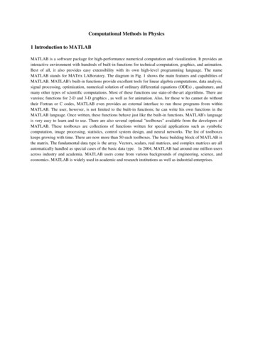
Figure 1.1: The graphical interface to the MATLAB workspace3
When MATLAB is started for the first time, the screen looks like the one that shownin the Figure 1.1. This illustration also shows the default configuration of the MATLABdesktop. You can customize the arrangement of tools and documents to suit your needs.Now, we are interested in doing some simple calculations. We will assume that youhave sufficient understanding of your computer under which MATLAB is being run.You are now faced with the MATLAB desktop on your computer, which contains the prompt( ) in the Command Window. Usually, there are 2 types of prompt: EDU for full versionfor educational versionNote: To simplify the notation, we will use this prompt, , as a standard prompt sign,though our MATLAB version is for educational purpose.1.3.2Using MATLAB as a calculatorAs an example of a simple interactive calculation, just type the expression you want toevaluate. Let’s start at the very beginning. For example, let’s suppose you want to calculatethe expression, 1 2 3. You type it at the prompt command ( ) as follows, 1 2*3ans 7You will have noticed that if you do not specify an output variable, MATLAB uses adefault variable ans, short for answer, to store the results of the current calculation. Notethat the variable ans is created (or overwritten, if it is already existed). To avoid this, youmay assign a value to a variable or output argument name. For example, x 1 2*3x 7will result in x being given the value 1 2 3 7. This variable name can alwaysbe used to refer to the results of the previous computations. Therefore, computing 4x willresult in 4*xans 28.0000Before we conclude this minimum session, Table 1.1 gives the partial list of arithmeticoperators.4
Table 1.1:Symbol /1.3.3Basic arithmetic operatorsOperationExampleAddition2 3Subtraction2 3Multiplication2 3Division2/3Quitting MATLABTo end your MATLAB session, type quit in the Command Window, or select File ExitMATLAB in the desktop main menu.1.4Getting startedAfter learning the minimum MATLAB session, we will now learn to use some additionaloperations.1.4.1Creating MATLAB variablesMATLAB variables are created with an assignment statement. The syntax of variable assignment isvariable name a value (or an expression)For example, x expressionwhere expression is a combination of numerical values, mathematical operators, variables,and function calls. On other words, expression can involve: manual entry built-in functions user-defined functions5
1.4.2Overwriting variableOnce a variable has been created, it can be reassigned. In addition, if you do not wish tosee the intermediate results, you can suppress the numerical output by putting a semicolon(;) at the end of the line. Then the sequence of commands looks like this: t 5; t t 1t 61.4.3Error messagesIf we enter an expression incorrectly, MATLAB will return an error message. For example,in the following, we left out the multiplication sign, *, in the following expression x 10; 5x? 5x Error: Unexpected MATLAB expression.1.4.4Making correctionsTo make corrections, we can, of course retype the expressions. But if the expression islengthy, we make more mistakes by typing a second time. A previously typed commandcan be recalled with the up-arrow key . When the command is displayed at the commandprompt, it can be modified if needed and executed.1.4.5Controlling the hierarchy of operations or precedenceLet’s consider the previous arithmetic operation, but now we will include parentheses. Forexample, 1 2 3 will become (1 2) 3 (1 2)*3ans 9and, from previous example6
1 2*3ans 7By adding parentheses, these two expressions give different results: 9 and 7.The order in which MATLAB performs arithmetic operations is exactly that taughtin high school algebra courses. Exponentiations are done first, followed by multiplicationsand divisions, and finally by additions and subtractions. However, the standard order ofprecedence of arithmetic operations can be changed by inserting parentheses. For example,the result of 1 2 3 is quite different than the similar expression with parentheses (1 2) 3.The results are 7 and 9 respectively. Parentheses can always be used to overrule priority,and their use is recommended in some complex expressions to avoid ambiguity.Therefore, to make the evaluation of expressions unambiguous, MATLAB has established a series of rules. The order in which the arithmetic operations are evaluated is givenin Table 1.2. MATLAB arithmetic operators obey the same precedence rules as those inTable 1.2: Hierarchy of arithmetic operationsPrecedence Mathematical operationsFirstThe contents of all parentheses are evaluated first, startingfrom the innermost parentheses and working outward.SecondAll exponentials are evaluated, working from left to rightThirdAll multiplications and divisions are evaluated, workingfrom left to rightFourthAll additions and subtractions are evaluated, startingfrom left to rightmost computer programs. For operators of equal precedence, evaluation is from left to right.Now, consider another example:14 6 22 35 7In MATLAB, it becomes 1/(2 3 2) 4/5*6/7ans 0.7766or, if parentheses are missing, 1/2 3 2 4/5*6/7ans 10.18577
So here what we get: two different results. Therefore, we want to emphasize the importanceof precedence rule in order to avoid ambiguity.1.4.6Controlling the appearance of floating point numberMATLAB by default displays only 4 decimals in the result of the calculations, for example 163.6667, as shown in above examples. However, MATLAB does numerical calculationsin double precision, which is 15 digits. The command format controls how the results ofcomputations are displayed. Here are some examples of the different formats together withthe resulting outputs. format short x -163.6667If we want to see all 15 digits, we use the command format long format long x -1.636666666666667e 002To return to the standard format, enter format short, or simply format.There are several other formats. For more details, see the MATLAB documentation,or type help format.Note - Up to now, we have let MATLAB repeat everything that we enter at theprompt ( ). Sometimes this is not quite useful, in particular when the output is pages enlength. To prevent MATLAB from echoing what we type, simply enter a semicolon (;) atthe end of the command. For example, x -163.6667;and then ask about the value of x by typing, xx -163.66671.4.7Managing the workspaceThe contents of the workspace persist between the executions of separate commands. Therefore, it is possible for the results of one problem to have an effect on the next one. To avoidthis possibility, it is a good idea to issue a clear command at the start of each new independent calculation.8
clearThe command clear or clear all removes all variables from the workspace. Thisfrees up system memory. In order to display a list of the variables currently in the memory,type whowhile, whos will give more details which include size, space allocation, and class of thevariables.1.4.8Keeping track of your work sessionIt is possible to keep track of everything done during a MATLAB session with the diarycommand. diaryor give a name to a created file, diary FileNamewhere FileName could be any arbitrary name you choose.The function diary is useful if you want to save a complete MATLAB session. Theysave all input and output as they appear in the MATLAB window. When you want to stopthe recording, enter diary off. If you want to start recording again, enter diary on. Thefile that is created is a simple text file. It can be opened by an editor or a word processingprogram and edited to remove extraneous material, or to add your comments. You canuse the function type to view the diary file or you can edit in a text editor or print. Thiscommand is useful, for example in the process of preparing a homework or lab submission.1.4.9Entering multiple statements per lineIt is possible to enter multiple statements per line. Use commas (,) or semicolons (;) toenter more than one statement at once. Commas (,) allow multiple statements per linewithout suppressing output. a 7; b cos(a), c cosh(a)b 0.6570c 548.31709
1.4.10Miscellaneous commandsHere are few additional useful commands: To clear the Command Window, type clc To abort a MATLAB computation, type ctrl-c To continue a line, type . . .1.4.11Getting helpTo view the online documentation, select MATLAB Help from Help menu or MATLAB Helpdirectly in the Command Window. The preferred method is to use the Help Browser. TheHelp Browser can be started by selecting the ? icon from the desktop toolbar. On the otherhand, information about any command is available by typing help CommandAnother way to get help is to use the lookfor command. The lookfor command differsfrom the help command. The help command searches for an exact function name match,while the lookfor command searches the quick summary information in each function fora match. For example, suppose that we were looking for a function to take the inverse ofa matrix. Since MATLAB does not have a function named inverse, the command helpinverse will produce nothing. On the other hand, the command lookfor inverse willproduce detailed information, which includes the function of interest, inv. lookfor inverseNote - At this particular time of our study, it is important to emphasize one main point.Because MATLAB is a huge program; it is impossible to cover all the details of each functionone by one. However, we will give you information how to get help. Here are some examples: Use on-line help to request info on a specific function help sqrt In the current version (MATLAB version 7), the doc function opens the on-line versionof the help manual. This is very helpful for more complex commands. doc plot10
Use lookfor to find functions by keywords. The general form is lookfor FunctionName1.5ExercisesNote: Due to the teaching class during this Fall 2005, the problems are temporarily removedfrom this section.11
Chapter 2Tutorial lessons 22.1Mathematical functionsMATLAB offers many predefined mathematical functions for technical computing whichcontains a large set of mathematical functions.Typing help elfun and help specfun calls up full lists of elementary and specialfunctions respectively.There is a long list of mathematical functions that are built into MATLAB. Thesefunctions are called built-ins. Many standard mathematical functions, such as sin(x), cos(x),tan(x), ex , ln(x), are evaluated by the functions sin, cos, tan, exp, and log respectively inMATLAB.Table 2.1 lists some commonly used functions, where variables x and y can be numbers,vectors, or matrices.Table 2.1: Elementary p(x)sqrt(x)log(x)log10(x)CosineSineTangentArc cosineArc sineArc tangentExponentialSquare rootNatural logarithmCommon ound(x)rem(x)angle(x)conj(x)Absolute valueSignum functionMaximum valueMinimum valueRound towards Round towards Round to nearest integerRemainder after divisionPhase angleComplex conjugateIn addition to the elementary functions, MATLAB includes a number of predefined12
constant values. A list of the most common values is given in Table 2.2.Table 2.2: Predefined constant valuespii,jInfNaN2.1.1The π number, π 3.14159. The imaginary unit i, 1The infinity, Not a numberExamplesWe illustrate here some typical examples which related to the elementary functions previouslydefined. As a first example, the value of the expression y e a sin(x) 10 y, for a 5, x 2, andy 8 is computed by a 5; x 2; y 8; y exp(-a)*sin(x) 10*sqrt(y)y 28.2904The subsequent examples are log(142)ans 4.9558 log10(142)ans 2.1523Note the difference between the natural logarithm log(x) and the decimal logarithm (base10) log10(x).To calculate sin(π/4) and e10 , we enter the following commands in MATLAB, sin(pi/4)ans 0.7071 exp(10)ans 2.2026e 00413
Notes: Only use built-in functions on the right hand side of an expression. Reassigning thevalue to a built-in function can create problems. There are some exceptions. For example, i and j are pre-assigned to 1. However,one or both of i or j are often used as loop
you learn quickly the flrst steps. The emphasis here is \learning by doing". Therefore, the best way to learn is by trying it yourself. Working through the examples will give you a feel for the way that MATLAB operates. In this introduction we will describe how MATLAB handle