Transcription
ECE 115Introduction to Electrical and Computer EngineeringLaboratory Experiment #1Using the MATLAB Desktop and Command WindowIn this experiment you will learn: how to start and quit MATLAB, about the organizationof the MATLAB desktop and command window, how to enter instructions for immediateexecution, some MATLAB syntax, how to define the complex number and matrix data type, howto do complex arithmetic, compute with vectors, use MATLAB plotting functions, and how touse the help facility.A Brief History of Computer TechnologyA complete history of computing would include a multitude of diverse devices such asthe ancient Chinese abacus, the Jacquard loom (1805) and Charles Babbage's analytical engine''(1834). It would also include discussion of mechanical, analog and digital computingarchitectures. As late as the 1960s, mechanical devices, such as the Marchant calculator, stillfound widespread application in science and engineering. During the early days of electroniccomputing devices, there was much discussion about the relative merits of analog vs. digitalcomputers. In fact, as late as the 1960s, analog computers were routinely used to solve systemsof finite difference equations arising in oil reservoir modeling. In the end, digital computingdevices proved to have the power, economics and scalability necessary to deal with large scalecomputations. Digital computers now dominate the computing world in all areas ranging fromthe hand calculator to the supercomputer and are pervasive throughout society.The evolution of digital computing is often divided into generations. Each generation ischaracterized by dramatic improvements over the previous generation in the technology used tobuild computers, the internal organization of computer systems, and the programming languages.The Mechanical Era (1623-1945)The idea of using machines to solve mathematical problems can be traced at least as farback as the early 17th century. The first multi-purpose, i.e., programmable, computing devicewas probably Charles Babbage's Difference Engine, which was built beginning in 1823, but wasnever completed. A more ambitious machine was the Analytical Engine. It was designed in1842, but unfortunately it also was only partially completed by Babbage. Babbage was truly aman ahead of his time: many historians think the major reason he was unable to complete theseprojects was the fact that the technology of the day was not reliable enough. A machine inspiredby Babbage's design was arguably the first to be used in computational science. George Scheutzread of the difference engine in 1833, and along with his son Edvard Scheutz began work on asmaller version. By 1853 they had constructed a machine that could process 15-digit numbers
and calculate fourth-order differences. Their machine won a gold medal at the Exhibition ofParis in 1855, and later they sold it to the Dudley Observatory in Albany, New York, which usedit to calculate the orbit of Mars. One of the first commercial uses of mechanical computers wasby the US Census Bureau, which used punch-card equipment designed by Herman Hollerith totabulate data for the 1890 census. In 1911 Hollerith's company merged with a competitor tofound the corporation which in 1924 became International Business Machines.First Generation Electronic Computers (1937-1953)Three machines have been promoted at various times as the first electronic computers.These machines used electronic switches, in the form of vacuum tubes, instead ofelectromechanical relays. Electronic components had one major benefit-they could open'' and close'' about 1,000 times faster than mechanical switches.The earliest attempt to build an electronic computer was by J. V. Atanasoff, a professorof physics and mathematics at Iowa State, in 1937. Atanasoff set out to build a machine thatwould help his graduate students solve systems of partial differential equations. By 1941 he andgraduate student Clifford Berry had succeeded in building a machine that could solve 29simultaneous equations with 29 unknowns. However, the machine was not programmable, andwas more of an electronic calculator.A second early electronic machine was Colossus, designed by Alan Turing for the Britishmilitary in 1943. This machine played an important role in breaking codes used by the Germanarmy in World War II. Turing's main contribution to the field of computer science was the ideaof the Turing machine, a mathematical formalism widely used in the study of computablefunctions. The existence of Colossus was kept secret until long after the war ended, and thecredit due to Turing and his colleagues for designing one of the first working electroniccomputers was slow in coming.The first general purpose programmable electronic computer was the ElectronicNumerical Integrator and Computer (ENIAC), built by J. Presper Eckert and John V. Mauchly atthe University of Pennsylvania. Work began in 1943, funded by the Army Ordnance Department,which needed a way to compute ballistics during World War II. The machine wasn't completeduntil 1945, but then it was used extensively for calculations during the design of the hydrogenbomb.Software technology during this period was very primitive. The first programs werewritten in machine code, i.e., programmers directly wrote down the binary numbers thatcorresponded to the instructions they wanted to store in memory. By the 1950s programmerswere using a symbolic notation, known as assembly language, then hand-translated the symbolicnotation into machine code. Later programs known as assemblers performed the translation task.Second Generation (1954-1962)The second generation saw several important developments at all levels of computersystem design, from the technology used to build the basic circuits to the programminglanguages used to write scientific applications.Electronic switches in this era were based on discrete diode and transistor technologywith a switching time of approximately 0.3 microseconds. The first machines to be built with this
technology include TRADIC at Bell Laboratories in 1954 and TX-0 at MIT's LincolnLaboratory.During this second generation, many high level programming languages were introduced,including FORTRAN (1956), ALGOL (1958), and COBOL (1959). The second generation alsosaw the first two supercomputers designed specifically for numeric processing in scientificapplications.Third Generation (1963-1972)The third generation brought huge gains in computational power. Innovations in this erainclude the use of integrated circuits, or ICs (semiconductor devices with several transistors builtinto one physical component), semiconductor memories started to be used instead of magneticcores, and the introduction of operating systems.The first ICs were based on small-scale integration (SSI) circuits, which had around 10basic logic devices per circuit (or chip''), and evolved to the use of medium-scale integrated(MSI) circuits, which had up to 100 basic logic devices per chip.Fourth Generation (1972-1984)The next generation of computer systems saw the use of large scale integration (LSI 1000 devices per chip) and very large scale integration (VLSI - 100,000 devices per chip) in theconstruction of computing elements. Semiconductor memories replaced core memories as themain memory in most systems.Two important events marked the early part of the fourth generation: the development ofthe C programming language and the UNIX operating system, both at Bell Labs. In 1972, DennisRitchie developed the C language. C was then used to write a version of UNIX. This C-basedUNIX was soon ported to many different computers, relieving users from having to learn a newoperating system each time they change computer hardware. UNIX or a derivative of UNIX isnow a de facto standard on virtually every computer system.Fifth Generation (1984-1990)The fifth generation saw the introduction of machines with hundreds of processors thatcould all be working on different parts of a single program. The scale of integration insemiconductors continued at an incredible pace - by 1990 it was possible to build chips with amillion components - and semiconductor memories became standard on all computers.Other new developments were the widespread use of computer networks and theincreasing use of single-user workstations. This period also saw a marked increase in both thequality and quantity of scientific visualization.Sixth Generation (1990 - )This generation began with many gains in parallel computing, both in the hardware areaand in improved understanding of how to develop algorithms to exploit diverse, massivelyparallel computer architectures.
One of the most dramatic changes in the sixth generation has been the explosive growthof wide area networking. Network bandwidth has expanded tremendously in the last few yearsand will continue to improve for the next several years.110001000101011100010100x -2.0;11000101000111elsedisp('press enter')pauseendpress 101110100011011100010100000110001110Illustration of the computing processBefore you come to the laboratory, read the chapter, MATLAB Environment, that was puton the blackboard.For this experiment, you will be using MATLAB that is installed in the computers located in thelab.1) Click on the MATLAB icon to launch MATLAB. The window shown is the MATLABdesktop window. Within the tool bar at the top of the desktop there are the file, edit, view, etc.tools, and on the bar below the tool bar there is a little window that shows the current directorywhere MATLAB will retrieve and store files. This directory can be changed by clicking on thebutton to the right of the current directory window. If it is not already open, click on the viewtool button, and open and activate the command window.a) Type into the command window: " 2 3 . 5 "(do not type the quotation marks.), and pressenter. Explain what happened? You can also assign a value to a variable. Type into thecommand window: " x 2 3.5" , and press enter. Explain what happened. To prevent animmediate display of a calculation result, end the input with a semi-colon.Type:" y 3 2 log( pi / 2)*sin( x); " , and press enter. What value did MATLAB use for x? To seethe result, type: " y " , and explain what happened.b) MATLAB has an enormous number of built in functions. Type: "theta a sin( 0.5)" , andexplain what happened. Click on the HELP tool in the tool bar at the top of the commandwindow, and select Product Help. When the help window opens, click on the Search Results tabat the left. Type in: “tan”, and select it. On the right of the help window MATLAB will showhow to use the built in tangent function. In the command window, type in an expression toobtain the tangent of: / 3 . Give the MATLAB expression, and explain what happened.c) MATLAB can output results in different formats. Type in: “format short e”. Then type: “pi”,which is a word reserved by MATLAB to mean 3.14159 . What happened? Now type:“format long”, and then type: “pi”. What happened? Repeat the above for: ”format long e”.What happened? Then, return the format to: “format short”.
d) Use MATLAB to obtain the results for:24 / (24 1); sqrt (7); ln(e2 ); log10 (104 ); y cosh 2 (4.2 )Use the help facility of MATLAB to find out how to use the built-in functions given here. Giveyour MATLAB statements and results.e) MATLAB can work with complex numbers. It uses the letters, “j” and “i” to mean 1 . Toassign the complex number: -3-j4 to the variable x, write the MATLAB statement: “x -3-j*4” .Type in: “z -3 j*4 ”. What happened? Repeat for: “a cos(3*pi/2)-j*sin(3*pi/2)”. Explainwhy the result has a real part that is zero.f) Use MATLAB to compute: (-3.5-j5))/(1.7-j4). Give the MATLAB statement and result.2) MATLAB is ideally suited to work with vectors and matrices. A matrix is an array ofelements, such as: 3 5 1 a 3.5 6 7 Here, the matrix, a, has 2 rows and 3 columns, and the element in the first row and secondcolumn is a12 5. With subscripts we can refer to any element in the array (matrix). Generally,we write: X n m to refer to the element in the nth row and mth column. Of course, we could writeinstead: X k l to refer to an element in the matrix X. The dimension of a matrix gives the size ofthe matrix, and here the dimension is the number of rows and columns in the matrix. For thematrix a, the dimension is a 2x3 matrix. An Nx1 matrix is an N element column vector, and a1xM matrix is an M element row vector. A matrix can have more than two dimensions. A threedimensional matrix would have a size given by, for example, N x M x K, for some integers N, Mand K.a) Type in: " x 2 3 4 " . What happened? To assign a row vector to a variable, we canput a blank between each element in the assignment statement. Type in: " y 3; 1; 6; " .What happened? What is the dimension of y? A semi-colon terminates a row definition, andstarts a new row.b) Write a MATLAB statement to assign to z a row vector with elements: z11 3 , z12 5 , andz13 1.5 . What happens when you type: “a x z”? What corresponding elements of x and zwere summed? What happens when you type: “b x y”, and explain? Give the result for:b 2*a, and explain.c) MATLAB has many convenient functions to define a matrix. Type in: “x linspace(0, 9, 4)”.What happened? Use the MATLAB help facility to look up the function, linspace. Give anexplanation for what this function does.d) Type in: “z sqrt(x)”, where x was defined in part (c). Explain the result. What does eachelement of z mean? Repeat this for: x , and explain the result.e) MATLAB is very useful for matrix algebra. To multiply two vectors, let us use for example,x 2 4 3 , and a 2 5 4 . Type them into MATLAB. Now, compute y (a)(xtranspose), by typing: “y a*x’ “, where the prime takes the transpose of x, making x’ a columnvector. Explain the result. Here, we have computed the inner product of two vectors.
e) To multiply the corresponding elements of two matrices, use the operation “.*” . Type in:“y x.*a”. Explain the result.f) Type in: “y a’*x”, which multiplies the column vector a’ times the row vector x. Explain theresult. Here, we have computed the outer product of two vectors.g) Write MATLAB statements to find y for each element in x, where an element, x n , of x isgiven by: xn n / 2, n 0, 1, ., 10 , and y 1.5 x 6.25 . Give the result.3) MATLAB has many built-in functions for plotting. Type in the following statements. Note, inplace of names, enter your names.clear allclcf 50;T0 1/f;w 2*pi*f;N 200;time linspace(0, 4.0*T0, N 1);x cos(w*time);plot(time,x)xlabel('time - seconds')ylabel('volts')title('Sinusoidal Function, Names')a) Explain each line. Type in the variable names: T0, f, w, and N and give their values.b) Type in grid on. Explain what happened.c) In the figure window, use the file pull down menu to print the figure and include it in yourlab report.d) How many cycles of the sinusoidal function does your figure show?e) In milli seconds, give the time in which the sinusoidal function goes through one cycle.f) If you heard a sound that could be caused by this sinusoidal function, would you say thatthe sound is a low or a high frequency sound? Give an example of a musical instrument in aband that mainly produces sounds having the frequencies like this sinusoidal function.
ECE 115Introduction to Electrical and Computer EngineeringLaboratory Experiment #2Matrices, Vectors, Complex Numbers and ProgramsIn this experiment you will learn about several MATLAB built-in functions, matrix andvector operations and the complex number data type. Shown below are several MATLABprograms. You will learn how each program works and how to modify it as specified.Before you come to lab, read Sections 1 and 2 of Chapter 2, titled, "Programsand Functions".ExperimentIn all of the following programs use MATLAB help to find out about the kind of operation andbuilt-in function.% Your experiment report must provide a print of the program and the results.% Make a separate program, m-file, for each problem.% Name the files PROB1.m, PROB2.m, and so on.%% Problem 1clear all;f 2.0;w 2.0*pi*f;time [0.0:0.01:2.0]; %line 9amp 5.0;phase pi/4.0;x amp*cos(w*time phase); %line 12plot(time,x);grid on;title('Cosine Function'); %line 15disp('press enter to continue'); pause; %this appears in the Command Window%% a) Explain what line 9 does. Add a statement that uses the MATLAB, size,%function to find out how many entries the matrix, time, has. Do this%again, but use the MATLAB function, length.% b) Explain what line 12 does.% c) Add statements after line 15 to put axis labels on the plot.% Use volts for the vertical axis, and use seconds for the horizontal axis.%% Problem 2clear all;a -3.0;b 6.5;
c1 a i*b; %line 27real c1 real(c1);imag c1 imag(c1);mag c1 abs(c1); %line 30angle c1 angle(c1);%c2 3.0*exp(i*pi/4); %line 33%% a) Explain what line 27 does, and give the value of c1.%Add a MATLAB statement to find c2 the complex conjugate of c1.%Use the MATLAB help facility to find out about the MATLAB%function to obtain the complex conjugate of a complex number.% b) Explain what line 30 does.% c) Explain what line 33 does.%N 10; T 0.01;time [-N*T:T:N*T]; % line 40w pi/4.0;z 2.0*exp(i*w*time); x real(z); %line 42plot (time,x);grid on; %line 44disp('press enter to continue'); pause;%% d) Explain what line 40 does.% e) Explain what line 42 does. Is z a real or complex vector? What%is the dimension of z?% f) Add title and axes statements after line 44, and run the program.%Provide program and result print out.% g) Add statements to find and plot the imaginary part of z, and run%the program. Provide program and result print out.%% Problem 3clear all;p1 [1.0 1.0 -2.0]; %line 52r p1 roots(p1); disp(r p1); %line 53disp('press enter to continue'); pause; % Use HELP to find out about pause.p2 [3.0 4.5 -1.5 20.0];r p2 roots(p2); disp(r p2);disp('press enter to continue'); pause;p3 poly(r p2); %line 58%% a) Explain what line 52 does.% b) Explain what line 53 does. Look up the roots function.% c) Explain line 58, and explain results. Add a statement to display p3.% d) Add statements to find roots of: x 3 2.0*x 2 2.0*x 1 1.0 0.0.% e) Add statements to verify your results of part (d), i.e., use a MATLAB%function to find a polynomial given its roots.%% Problem 4clear all;a [1.0 1.0; 1.5 2.0]; %line 68d a'; %line 69b inv(a); %line 70c a*b; %line 71disp(c);disp('press enter to continue'); pause;%
% a) Explain what line 68 does.% b) Explain what line 69 does.% c) Explain what line 70 does. Manually find the inverse of A, and%check program results.% d) Explain what line 71 does, and explain the results.% d) Add statements to solve equation: a*x y, for x, where y [1.0 3.0]'.%% Problem 5clear all;% A [1 2 3; 4 5 6; 7 8 9]% The above line defines a 3x3 matrix. We can use MATLAB continuation andwriteA [1 2 3; .4 5 6; .7 8 9]; % The three dots cause a line to be continuedb A(2,3) %line 88, get an elementC A(2:3, 1:3) % line 89, get rows 2 and 3 from columns 1 to 3D A(1:2, :) % line 90, get rows 1 and 2 from all columnsD(:, 2) [] % line 91, delete column 2 in all rows by nulling column 2v [10 11 12];E [A v'] % line 93, augment A with a columnF [A; v] % line 94, augment A with a row[m, n] size(E) % line 95G zeros(m,n) % line 96%% a) Explain what line 88 does.% b) Explain what line 89 does.% c) Explain what line 90 does.% d) Explain what line 91 does.% e) Explain what line 92 does.% f) Explain what line 93 does.% g) Explain what line 94 does.% h) Explain what line 95 does.% i) Explain what line 96 does.%% Problem 6% We see that MATLAB has numerous methods to manipulate vectors and matrices% Use MATLAB help to describe the following operations (built-in functions):%% a)eye(m,n)% b)ones(m,n)% c)rand(m,n)% d)diag(v)% e)fliplr% f)flipud%% g) and give a program that illustrates the use of each of these operations.%% Problem 7% In MATLAB vectors can be created in many ways.clear all;v begin -1.0;v end 12.0;v linspace(v begin, v end, 14) % line 126u zeros(1, 100) % line 127w ones(1, 10) % line 128x -1.0:2:20 % line 129
theta 0:pi/16:2*pi; k size(theta) % line 130%% a) Explain what line 126 does.% b) Explain what line 127 does.% c) Explain what line 128 does.% d) Explain what line 129 does.% e) Explain what line 130 does.%% Problem 8clear all;a [10 2 3 4 5; .6 7 8 9 10; .0 -1 -2 -3 -4; .-5 -6 -7 -8 9; .1 2 3 2 1];b [-1 -3 4 5 2; .3 7 5 9 5; .-1 -2 -3 -4 0; .5 -2 -1 2 0; .3 2 -1 0 1];c a/b % line 150d det(a)e det(b) % line 152f det(c); g d/e;fg%% a) Explain what line 150 does.% b) Explain what line 152 does.% c) Why are f and g equal, explain?Problem 9Look up the arc-tangent (atan) function, and write a program to plot it: y atan(x), with 501points over the range: x -100.0 to 100.0. Provide a program listing and a plot.
ECE 115Introduction to Electrical and Computer EngineeringLaboratory Experiment #3Loops, Branches and Program Flow ControlObjective: To learn about and how to use MATLAB program flow control commands.in p u tif( i 1)r0ebrkmenu0000umRileturn pauendoarda n s in p u t( 'Y e s /N o ','s ')eaileybsel whFOkesennuin p u trewh 2(j if&xoelu(semeifwh ile npa0)ileee lsrd 5)end oa Rwhr 1 FO fo0)yb&(y key )& (x e rrin p u to r('insechoee l sc o l o ridvalic e')Before you come to the Lab, read Sections 1-5 of Chapter 4, titled, “ProgramFlow Control”, which is posted on the blackboard.For processing certain operations and commands repeatedly, MATLAB has for loop andwhile loop commands. With the if-elseif-else structure a program can test conditions andexecute alternative program segments. With the break, error, and return commands programexecution can be controlled. Interactive input is facilitated with the input, keyboard, menu andpause commands. These commands are often used in association with relational and logicaloperations, which produce a logical result. In this experiment you will learn about each of thesecommands and to use relational and logical operations.The relational operations are: less than less than or equal to greater than
greater than or equal toequal tonot equal toand the logical operations are:&and or notxorexclusive or functionA relational operation produces either 1, meaning the relation is true, or 0, meaning the relationis false. For example, consider the following MATLAB program segment:x 2.0;y -5.0;z1 x y;z2 x y;z3 x y;The result is: z1 0, since it is not true (false) that x is less than y, z2 0, since it is false that xequals y, and z3 1, since it is true that x is not equal to y. Relational operations and logicaloperations can be compounded. For example, the following MATLAB program segment:w 9.0; x 2.0; y -5.0;z1 (x y) & (x w);produces z1 1, since it is true that x is greater than y, and it is true that x is less than w. If theexpression is instead: z1 (x y) & (x w), then z1 0, since (x w) is true, and (x w) is false.EXPERIMENTFor each of the following problems, your report should include a listing of your program.Problem 1a) Type in the following for loop.sum 0.0;for m 0:2:8sum sum 1/(2 m);endsumWhat is the value of m and sum after the loop has executed?b) Type in the following program.
for n 10:-2:-10, k 1/exp(n), endDescribe how n changes through each loop. What is the purpose of the commas? Whathappens if commas are replaced by semi-colons?Problem 2a) Type in the following program.% find all powers of two below Nclear allN 500;v 1; num 1; i 1;while num Nnum 2 i;v [v; num]; % explain this linei i 1;endv % display vWhat is the dimension of v after this program has executed?b) Modify the program of part (a) so that a user of the modified program is instructed to enter avalue for N. Execute the program only if an N greater than two is entered. If N is not greaterthan two inform the user that the program will be terminated. Use a while loop around thepresent while loop. For example, you could start with:N input(‘Enter a value for N: ‘)go N 1;while goy 1;.Test your program for N greater than and less than 2, and describe results. Look up the inputcommand in MATLAB help, and discuss what the input command does when ‘s’ is alsoincluded in the input statement.For example, consider the following MATLAB program segment.clear allx input('enter Y/N: ','s')ans (x 'Y') (x 'y')Explain what this program segment does, and specifically, explain what is being comparedwith the operations.Problem 3
a) Type in the following program.clear all;a 2; j 21;if a 5k a;elseif (a 1) & (j 20)k 5 * a j;elsek 1;endHere, in the if command, MATLAB checks whether or not, a 5, is true, and if it is true, then k ais executed, and then execution continues after the end statement. However, if a 5 is false, thenin the next elseif command, (a 1) & (j 20), is checked, and if it is true then the nextstatement, k 5 * a j, is executed and execution continues after the end command, and if it isfalse, then the statement, k 1, after the else command, is executed. Any number of additionalelseif sections can be added. Add another elseif section to the program that executes, k j,if a 1. Then, for what assignment to a can it occur that k 1 results?b) The command break inside a for or a while loop unconditionally terminates the execution ofthe loop. Just before the statement, i i 1, in the program of part (2a) add the statements:if length(v) 8breakendUse MATLAB help to find out what the length command does, and explain what happens inthe program due to the addition of the above statements.c) Write a small program that uses a while loop that includes within it an if-end structure likethe one given above to break out of the while loop. Explain program operation.Problem 4The command error(‘message’) terminates function or program execution and returns control tothe keyboard. The return command returns control from a function back to the invokingprogram or function. The keyboard command inside a function or program returns control tothe keyboard at the point where the keyboard command occurs. Within the command windowthe prompt becomes k to show that the keyboard command has executed. Any validMATLAB command can then be executed from within the command window. Program orfunction execution can be made to continue just after the place where the keyboard commandoccurs by entering the return command from within the command window.Write a program to use the following function, and describe what happened when yourprogram executes a statement like b SquareRoot(a) for a 2, a 0 and a -1.
function y SquareRoot(x);y 0;if x 0error('the function argument cannot be negative')endif x 0returnelsey x 0.5;endProblem 5a) The following program illustrates use of the menu command.clear alltheta linspace(0, 2.0*pi, 101);x sin(theta);plot type menu('plot type menu','stem plot','line plot'); % display plot selection menuif plot type 1stem(theta, x);elseplot(theta,x);endgrid ondisp('press enter to continue'); pause; % pause to view plotType in the program given above, and execute it. Describe the appearance of the menu. Selecteach menu item and describe what the program does. What does the pause command do?b) Add another type of plot choice to the menu command, and expand the if-end structure withan elseif segment to include the new plot type in the possible output plots.
ECE 115Introduction to Electrical and Computer EngineeringLaboratory Experiment #4Use of Some Analog InstrumentationThe purpose of this experiment is to become acquainted with the operation and utility ofsome of the conventional instrumentation used to investigate the operation of electroniccircuits and devices. You will learn how to use an oscilloscope, a signal (function)generator, a multimeter, a power supply, and a facility for conveniently putting togethersmall circuits.OscilloscopeThe oscilloscope, like the one shown below, is probably the most widely usedinstrument to investigate the operation of an electronic circuit. The oscilloscopeprovides a visual display of the voltage between two points in an electronic circuit, asthis voltage varies with time.
This oscilloscope can display simultaneously two voltages, one voltage that is aninput to its channel 1 input and another voltage that is an input to its channel 2 input.The user can elect to view either channel 1 or channel 2, or both. Basically, the way anoscilloscope (scope) works is very simple. Electronic circuitry within the scope controlsthe horizontal position of a lighted point on the display screen. This lighted point ismade to repeatedly sweep across the display screen from left to right, giving theappearance of a horizontal line to the observer. The voltage that is applied at an inputto a channel causes the lighted point to be deflected up, if the input voltage is positive,or down, if the input voltage is negative. Therefore, as the lighted point sweeps acrossthe display screen, the viewer will observe a lighted wave shape that corresponds tohow the channel input voltage varies with time.There are many attributes of how the observed wave shape should appear onthe display, and that is why there are many controls on the front panel of a scope.Some of these controls are set according to user preferences, such as: the horizontalwidth of the displayed image, the vertical position of the displayed wave shape, theintensity (brightness) of the display, and others. Some of these controls are setaccording to what the voltage to be displayed is like.For example, if the input voltage varies very slowly with time and the lighted pointsweeps across the display very quickly, then the image looks more-or-less like ahorizontal line, and we do not see very well how the input voltage varies with time. Inthis case we would adjust a front panel control to decrease the horizontal swe
of the MATLAB desktop and command window, how to enter instructions for immediate execution, some MATLAB syntax, how to define the complex number and matrix data type, how to do complex arithmetic, compute with vectors, use MATLAB plotting functions, and how to use the help facility