Transcription
scikit-learn#scikit-learn
Table of ContentsAbout1Chapter 1: Getting started with scikit-learn2Remarks2Examples2Installation of scikit-learn2Train a classifier with cross-validation2Creating pipelines3Interfaces and conventions:4Sample datasets4Chapter 2: ClassificationExamples66Using Support Vector Machines6RandomForestClassifier6Analyzing Classification Reports7GradientBoostingClassifier8A Decision Tree8Classification using Logistic Regression9Chapter 3: Dimensionality reduction (Feature selection)ExamplesReducing The Dimension With Principal Component AnalysisChapter 4: Feature selectionExamplesLow-Variance Feature RemovalChapter 5: Model 5K-Fold Cross Validation15K-Fold16ShuffleSplit16Chapter 6: Receiver Operating Characteristic (ROC)17
Examples17Introduction to ROC and AUC17ROC-AUC score with overriding and cross validation18Chapter 7: RegressionExamplesOrdinary Least SquaresCredits20202022
AboutYou can share this PDF with anyone you feel could benefit from it, downloaded the latest versionfrom: scikit-learnIt is an unofficial and free scikit-learn ebook created for educational purposes. All the content isextracted from Stack Overflow Documentation, which is written by many hardworking individuals atStack Overflow. It is neither affiliated with Stack Overflow nor official scikit-learn.The content is released under Creative Commons BY-SA, and the list of contributors to eachchapter are provided in the credits section at the end of this book. Images may be copyright oftheir respective owners unless otherwise specified. All trademarks and registered trademarks arethe property of their respective company owners.Use the content presented in this book at your own risk; it is not guaranteed to be correct noraccurate, please send your feedback and corrections to info@zzzprojects.comhttps://riptutorial.com/1
Chapter 1: Getting started with scikit-learnRemarksis a general-purpose open-source library for data analysis written in python. It isbased on other python libraries: NumPy, SciPy, and matplotlibscikit-learnscikit-learncontainsa number of implementation for different popular algorithms of machinelearning.ExamplesInstallation of scikit-learnThe current stable version of scikit-learn requires: Python ( 2.6 or 3.3), NumPy ( 1.6.1), SciPy ( 0.9).For most installation pip python package manager can install python and all of its dependencies:pip install scikit-learnHowever for linux systems it is recommended to use conda package manager to avoid possiblebuild processesconda install scikit-learnTo check that you have scikit-learn, execute in shell:python -c 'import sklearn; print(sklearn. version )'Windows and Mac OSX Installation:Canopy and Anaconda both ship a recent version of scikit-learn, in addition to a large set ofscientific python library for Windows, Mac OSX (also relevant for Linux).Train a classifier with cross-validationUsing iris dataset:import sklearn.datasetsiris dataset sklearn.datasets.load iris()https://riptutorial.com/2
X, y iris dataset['data'], iris dataset['target']Data is split into train and test sets. To do this we use the train test split utility function to splitboth X and y (data and target vectors) randomly with the option train size 0.75 (training setscontain 75% of the data).Training datasets are fed into a k-nearest neighbors classifier. The method fit of the classifier willfit the model to the data.from sklearn.cross validation import train test splitX train, X test, y train, y test train test split(X, y, train size 0.75)from sklearn.neighbors import KNeighborsClassifierclf KNeighborsClassifier(n neighbors 3)clf.fit(X train, y train)Finally predicting quality on test sample:clf.score(X test, y test) # Output: 0.94736842105263153By using one pair of train and test sets we might get a biased estimation of the quality of theclassifier due to the arbitrary choice the data split. By using cross-validation we can fit of theclassifier on different train/test subsets of the data and make an average over all accuracy results.The function cross val score fits a classifier to the input data using cross-validation. It can take asinput the number of different splits (folds) to be used (5 in the example below).from sklearn.cross validation import cross val scorescores cross val score(clf, X, y, cv 5)print(scores)# Output: array([ 0.96666667, 0.96666667, 0.93333333, 0.96666667, 1.print "Accuracy: %0.2f ( /- %0.2f)" % (scores.mean(), scores.std() / 2)# Output: Accuracy: 0.97 ( /- 0.03)])Creating pipelinesFinding patterns in data often proceeds in a chain of data-processing steps, e.g., feature selection,normalization, and classification. In sklearn, a pipeline of stages is used for this.For example, the following code shows a pipeline consisting of two stages. The first scales thefeatures, and the second trains a classifier on the resulting augmented dataset:from sklearn.pipeline import make pipelinefrom sklearn.preprocessing import StandardScalerfrom sklearn.neighbors import KNeighborsClassifierpipeline make pipeline(StandardScaler(), KNeighborsClassifier(n neighbors 4))Once the pipeline is created, you can use it like a regular stage (depending on its specific steps).Here, for example, the pipeline behaves like a classifier. Consequently, we can use it as follows:# fitting a classifierhttps://riptutorial.com/3
pipeline.fit(X train, y train)# getting predictions for the new data samplepipeline.predict proba(X test)Interfaces and conventions:Different operations with data are done using special classes.Most of the classes belong to one of the following groups: classification algorithms (derived from sklearn.base.ClassifierMixin) to solve classificationproblems regression algorithms (derived from sklearn.base.RegressorMixin) to solve problem ofreconstructing continuous variables (regression problem) data transformations (derived from sklearn.base.TransformerMixin) that preprocess the dataData is stored in numpy.arrays (but other array-like objects like pandas.DataFrames are accepted ifthose are convertible to numpy.arrays)Each object in the data is described by set of features the general convention is that data sampleis represented with array, where first dimension is data sample id, second dimension is feature id.import numpydata numpy.arange(10).reshape(5, 2)print(data)Output:[[0 1][2 3][4 5][6 7][8 9]]In sklearn conventions dataset above contains 5 objects each described by 2 features.Sample datasetsFor ease of testing, sklearn provides some built-in datasets in sklearn.datasets module. Forexample, let's load Fisher's iris dataset:import sklearn.datasetsiris dataset sklearn.datasets.load iris()iris dataset.keys()['target names', 'data', 'target', 'DESCR', 'feature names']You can read full description, names of features and names of classes (target names). Those arestored as strings.We are interested in the data and classes, which stored in data and target fields. By conventionthose are denoted as X and yhttps://riptutorial.com/4
X, y iris dataset['data'], iris dataset['target']X.shape, y.shape((150, 4), (150,))numpy.unique(y)array([0, 1, 2])Shapes of X and y say that there are 150 samples with 4 features. Each sample belongs to one offollowing classes: 0, 1 or 2.Xand y can now be used in training a classifier, by calling the classifier's fit() method.Here is the full list of datasets provided by the sklearn.datasets module with their size andintended use:Load withDescriptionSizeUsageload boston()Boston house-prices dataset506regressionload breast cancer()Breast cancer Wisconsin dataset569classification (binary)load diabetes()Diabetes dataset442regressionload digits(n class)Digits dataset1797classificationload iris()Iris dataset150classification (multi-class)load linnerud()Linnerud dataset20multivariate regressionNote that (source: http://scikit-learn.org/stable/datasets/):These datasets are useful to quickly illustrate the behavior of the various algorithmsimplemented in the scikit. They are however often too small to be representative of realworld machine learning tasks.In addition to these built-in toy sample datasets, sklearn.datasets also provides utility functions forloading external datasets: for loading sample datasets from the mlcomp.org repository (note that thedatasets need to be downloaded before). Here is an example of usage. fetch lfw pairs and fetch lfw people for loading Labeled Faces in the Wild (LFW) pairsdataset from http://vis-www.cs.umass.edu/lfw/, used for face verification (resp. facerecognition). This dataset is larger than 200 MB. Here is an example of usage.load mlcompRead Getting started with scikit-learn online: com/5
Chapter 2: ClassificationExamplesUsing Support Vector MachinesSupport vector machines is a family of algorithms attempting to pass a (possibly high-dimension)hyperplane between two labelled sets of points, such that the distance of the points from the planeis optimal in some sense. SVMs can be used for classification or regression (corresponding tosklearn.svm.SVC and sklearn.svm.SVR, respectively.Example:Suppose we work in a 2D space. First, we create some data:import numpy as npNow we create x and y:x0, x1 np.random.randn(10, 2), np.random.randn(10, 2) (1, 1)x np.vstack((x0, x1))y [0] * 10 [1] * 10Note that x is composed of two Gaussians: one centered around (0, 0), and one centered around(1, 1).To build a classifier, we can use:from sklearn import svmsvm.SVC(kernel 'linear').fit(x, y)Let's check the prediction for (0, 0): svm.SVC(kernel 'linear').fit(x, y).predict([[0, 0]])array([0])The prediction is that the class is 0.For regression, we can similarly do:svm.SVR(kernel 'linear').fit(x, y)RandomForestClassifierA random forest is a meta estimator that fits a number of decision tree classifiers on various subhttps://riptutorial.com/6
samples of the dataset and use averaging to improve the predictive accuracy and control overfitting.A simple usage example:Import:from sklearn.ensemble import RandomForestClassifierDefine train data and target data:train [[1,2,3],[2,5,1],[2,1,7]]target [0,1,0]The values in target represent the label you want to predict.Initiate a RandomForest object and perform learn (fit):rf RandomForestClassifier(n estimators 100)rf.fit(train, target)Predict:test [2,2,3]predicted rf.predict(test)Analyzing Classification ReportsBuild a text report showing the main classification metrics, including the precision and recall, f1score (the harmonic mean of precision and recall) and support (the number of observations of thatclass in the training set).Example from sklearn docs:from sklearn.metrics import classification reporty true [0, 1, 2, 2, 2]y pred [0, 0, 2, 2, 1]target names ['class 0', 'class 1', 'class 2']print(classification report(y true, y pred, target names target names))Output precisionrecallf1-scoresupportclass 0class 1class 20.500.001.001.000.000.670.670.000.80113avg / total0.700.600.615https://riptutorial.com/7
GradientBoostingClassifierGradient Boosting for classification. The Gradient Boosting Classifier is an additive ensemble of abase model whose error is corrected in successive iterations (or stages) by the addition ofRegression Trees which correct the residuals (the error of the previous stage).Import:from sklearn.ensemble import GradientBoostingClassifierCreate some toy classification datafrom sklearn.datasets import load irisiris dataset load iris()X, y iris dataset.data, iris dataset.targetLet us split this data into training and testing set.from sklearn.model selection import train test splitX train, X test, y train, y test train test split(X, y, test size 0.2, random state 0)Instantiate a GradientBoostingClassifier model using the default params.gbc GradientBoostingClassifier()gbc.fit(X train, y train)Let us score it on the test set# We are using the default classification accuracy score gbc.score(X test, y test)1By default there are 100 estimators built gbc.n estimators100This can be controlled by setting n estimators to a different value during the initialization time.A Decision TreeA decision tree is a classifier which uses a sequence of verbose rules (like a 7) which can beeasily understood.The example below trains a decision tree classifier using three feature vectors of length 3, andthen predicts the result for a so far unknown fourth feature vector, the so called test vector.https://riptutorial.com/8
from sklearn.tree import DecisionTreeClassifier# Define training and target set for the classifiertrain [[1,2,3],[2,5,1],[2,1,7]]target [10,20,30]# Initialize Classifier.# Random values are initialized with always the same random seed of value 0# (allows reproducible results)dectree DecisionTreeClassifier(random state 0)dectree.fit(train, target)# Test classifier with other, unknown feature vectortest [2,2,3]predicted dectree.predict(test)print predictedOutput can be visualized using:import pydotimport StringIOdotfile StringIO.StringIO()tree.export graphviz(dectree, out file dotfile)(graph,) pydot.graph from dot data(dotfile.getvalue())graph.write png("dtree.png")graph.write pdf("dtree.pdf")Classification using Logistic RegressionIn LR Classifier, he probabilities describing the possible outcomes of a single trial are modeledusing a logistic function. It is implemented in the linear model libraryfrom sklearn.linear model import LogisticRegressionThe sklearn LR implementation can fit binary, One-vs- Rest, or multinomial logistic regression withoptional L2 or L1 regularization. For example, let us consider a binary classification on a samplesklearn datasetfrom sklearn.datasets import make hastie 10 2X,y make hastie 10 2(n samples 1000)Where X is a n samplesX 10array and y is the target labels -1 or 1.Use train-test split to divide the input data into training and test sets (70%-30%)from sklearn.model selection import train test split#sklearn.cross validation in older scikit versionsdata train, data test, labels train, labels test train test split(X,y, test size 0.3)https://riptutorial.com/9
Using the LR Classifier is similar to other examples# Initialize Classifier.LRC LogisticRegression()LRC.fit(data train, labels train)# Test classifier with the test datapredicted LRC.predict(data test)Use Confusion matrix to visualise resultsfrom sklearn.metrics import confusion matrixconfusion matrix(predicted, labels test)Read Classification online: assificationhttps://riptutorial.com/10
Chapter 3: Dimensionality reduction (Featureselection)ExamplesReducing The Dimension With Principal Component AnalysisPrincipal Component Analysis finds sequences of linear combinations of the features. The firstlinear combination maximizes the variance of the features (subject to a unit constraint). Each ofthe following linear combinations maximizes the variance of the features in the subspaceorthogonal to that spanned by the previous linear combinations.A common dimension reduction technique is to use only the k first such linear combinations.Suppose the features are a matrix X of n rows and m columns. The first k linear combinations forma matrix βk of m rows and k columns. The product X β has n rows and k columns. Thus, theresulting matrix β k can be considered a reduction from m to k dimensions, retaining the highvariance parts of the original matrix X.In scikit-learn, PCA is performed with sklearn.decomposition.PCA. For example, suppose we startwith a 100 X 7 matrix, constructed so that the variance is contained only in the first two columns(by scaling down the last 5 columns):import numpy as npnp.random.seed(123) # we'll set a random seed so that our results are reproducibleX np.hstack((np.random.randn(100, 2) (10, 10), 0.001 * np.random.randn(100, 5)))Let's perform a reduction to 2 dimensions:from sklearn.decomposition import PCApca PCA(n components 2)pca.fit(X)Now let's check the results. First, here are the linear combinations:pca.components# array([[ -2.84271217e-01, -9.58743893e-01,#1.96237855e-05, -1.25862328e-05,#-9.46906600e-05],#[ -9.58743890e-01,2.84271223e-01,#-1.23188872e-04, 8.27127496e-05,-7.33055823e-05,5.50383246e-05,Note how the first two components in each vector are several orders of magnitude larger than theothers, showing that the PCA recognized that the variance is contained mainly in the first twocolumns.https://riptutorial.com/11
To check the ratio of the variance explained by this PCA, we can examinepca.explained variance ratio :pca.explained variance ratio# array([ 0.57039059, 0.42960728])Read Dimensionality reduction (Feature selection) online: iptutorial.com/12
Chapter 4: Feature selectionExamplesLow-Variance Feature RemovalThis is a very basic feature selection technique.Its underlying idea is that if a feature is constant (i.e. it has 0 variance), then it cannot be used forfinding any interesting patterns and can be removed from the dataset.Consequently, a heuristic approach to feature elimination is to first remove all features whosevariance is below some (low) threshold.Building off the example in the documentation, suppose we start withX [[0, 0, 1], [0, 1, 0], [1, 0, 0], [0, 1, 1], [0, 1, 0], [0, 1, 1]]There are 3 boolean features here, each with 6 instances. Suppose we wish to remove those thatare constant in at least 80% of the instances. Some probability calculations show that thesefeatures will need to have variance lower than 0.8 * (1 - 0.8). Consequently, we can usefrom sklearn.feature selection import VarianceThresholdsel VarianceThreshold(threshold (.8 * (1 - .8)))sel.fit transform(X)# Output: array([[0, 1],[1, 0],[0, 0],[1, 1],[1, 0],[1, 1]])Note how the first feature was removed.This method should be used with caution because a low variance doesn't necessarily mean that afeature is “uninteresting”. Consider the following example where we construct a dataset thatcontains 3 features, the first two consisting of randomly distributed variables and the third ofuniformly distributed variables.from sklearn.feature selection import VarianceThresholdimport numpy as np# generate datasetnp.random.seed(0)feat1 np.random.normal(loc 0, scale .1, size 100) # normal dist. with mean 0 and std .1feat2 np.random.normal(loc 0, scale 10, size 100) # normal dist. with mean 0 and std 10feat3 np.random.uniform(low 0, high 10, size 100) # uniform dist. in the interval [0,10)data np.column 13
data[:5]# Output:# array([[#[#[#[#[0.17640523, 18.83150697,0.04001572, -13.47759061,0.0978738 , -12.70484998,0.22408932,9.69396708,0.1867558 , -11.73123405,np.var(data, axis 0)# Output: array([ 1.01582662e-02,9.61936379],2.92147527],2.4082878 ],1.00293942],0.1642963 ]])1.07053580e 02,9.07187722e 00])sel VarianceThreshold(threshold 0.1)sel.fit transform(data)[:5]# Output:# array([[ ,#[-12.70484998,2.4082878 ],#[ 9.69396708,1.00293942],#[-11.73123405,0.1642963 ]])Now the first feature has been removed because of its low variance, while the third feature (that'sthe most uninteresting) has been kept. In this case it would have been more appropriate toconsider a coefficient of variation because that's independent of scaling.Read Feature selection online: ature-selectionhttps://riptutorial.com/14
Chapter 5: Model selectionExamplesCross-validationLearning the parameters of a prediction function and testing it on the same data is amethodological mistake: a model that would just repeat the labels of the samples that it has justseen would have a perfect score but would fail to predict anything useful on yet-unseen data. Thissituation is called overfitting. To avoid it, it is common practice when performing a (supervised)machine learning experiment to hold out part of the available data as a test set X test, y test.Note that the word “experiment” is not intended to denote academic use only, because even incommercial settings machine learning usually starts out experimentally.In scikit-learn a random split into training and test sets can be quickly computed with thetrain test split helper function. Let’s load the iris data set to fit a linear support vector machine onit: import numpyfrom sklearnfrom sklearnfrom sklearnas npimport cross validationimport datasetsimport svm iris datasets.load iris() iris.data.shape, iris.target.shape((150, 4), (150,))We can now quickly sample a training set while holding out 40% of the data for testing (evaluating)our classifier: X train, X test, y train, y test cross validation.train test split(.iris.data, iris.target, test size 0.4, random state 0) X train.shape, y train.shape((90, 4), (90,)) X test.shape, y test.shape((60, 4), (60,))Now, after we have train and test sets, lets use it: clf svm.SVC(kernel 'linear', C 1).fit(X train, y train) clf.score(X test, y test)K-Fold Cross ValidationK-fold cross-validation is a systematic process for repeating the train/test split procedure multipletimes, in order to reduce the variance associated with a single trial of train/test split. Youessentially split the entire dataset into K equal size "folds", and each fold is used once for testinghttps://riptutorial.com/15
the model and K-1 times for training the model.Multiple folding techniques are available with the scikit library. Their usage is dependent on theinput data characteristics. Some examples areK-FoldYou essentially split the entire dataset into K equal size "folds", and each fold is used once fortesting the model and K-1 times for training the model.from sklearn.model selection import KFoldX np.array([[1, 2], [3, 4], [5, 6], [7, 8]])y np.array([1, 2, 1, 2])cv KFold(n splits 3, random state 0)for train index, test index in cv.split(X):.print("TRAIN:", train index, "TEST:", test index)TRAIN: [2 3] TEST: [0 1]TRAIN: [0 1 3] TEST: [2]TRAIN: [0 1 2] TEST: [3]is a variation of k-fold which returns stratified folds: each set containsapproximately the same percentage of samples of each target class as the complete setStratifiedKFoldShuffleSplitUsed to generate a user defined number of independent train / test dataset splits. Samples arefirst shuffled and then split into a pair of train and test sets.from sklearn.model selection import ShuffleSplitX np.array([[1, 2], [3, 4], [5, 6], [7, 8]])y np.array([1, 2, 1, 2])cv ShuffleSplit(n splits 3, test size .25, random state 0)for train index, test index in cv.split(X):.print("TRAIN:", train index, "TEST:", test index)TRAIN: [3 1 0] TEST: [2]TRAIN: [2 1 3] TEST: [0]TRAIN: [0 2 1] TEST: [3]is a variation of ShuffleSplit, which returns stratified splits, i.e which createssplits by preserving the same percentage for each target class as in the complete set.StratifiedShuffleSplitOther folding techniques such as Leave One/p Out, and TimeSeriesSplit (a variation of K-fold) areavailable in the scikit model selection library.Read Model selection online: del-selectionhttps://riptutorial.com/16
Chapter 6: Receiver Operating Characteristic(ROC)ExamplesIntroduction to ROC and AUCExample of Receiver Operating Characteristic (ROC) metric to evaluate classifier output quality.ROC curves typically feature true positive rate on the Y axis, and false positive rate on the X axis.This means that the top left corner of the plot is the “ideal” point - a false positive rate of zero, anda true positive rate of one. This is not very realistic, but it does mean that a larger area under thecurve (AUC) is usually better.The “steepness” of ROC curves is also important, since it is ideal to maximize the true positiverate while minimizing the false positive rate.A simple example:import numpy as npfrom sklearn import metricsimport matplotlib.pyplot as pltArbitrary y values - in real case this is the predicted target values (model.predict(x test) ):y np.array([1,1,2,2,3,3,4,4,2,3])Scores is the mean accuracy on the given test data and labels (model.score(X,Y)):scores np.array([0.3, 0.4, 0.95,0.78,0.8,0.64,0.86,0.81,0.9, 0.8])Calculate the ROC curve and the AUC:fpr, tpr, thresholds metrics.roc curve(y, scores, pos label 2)roc auc metrics.auc(fpr, tpr)Plotting:plt.figure()plt.plot(fpr, tpr, label 'ROC curve (area %0.2f)' % roc auc)plt.plot([0, 1], [0, 1], 'k--')plt.xlim([0.0, 1.0])plt.ylim([0.0, 1.05])plt.xlabel('False Positive Rate')plt.ylabel('True Positive Rate')plt.title('Receiver operating characteristic example')plt.legend(loc "lower right")https://riptutorial.com/17
plt.show()Output:Note: the sources were taken from these link1 and link2ROC-AUC score with overriding and cross validationOne needs the predicted probabilities in order to calculate the ROC-AUC (area under the curve)score. The cross val predict uses the predict methods of classifiers. In order to be able to get theROC-AUC score, one can simply subclass the classifier, overriding the predict method, so that itwould act like predict proba.fromfromfromfromsklearn.datasets import make classificationsklearn.linear model import LogisticRegressionsklearn.cross validation import cross val predictsklearn.metrics import roc auc scoreclass s://riptutorial.com/18
def predict(self, X):return super(LogisticRegressionWrapper, self).predict proba(X)X, y make classification(n samples 1000, n features 10, n classes 2, flip y 0.5)log reg clf LogisticRegressionWrapper(C 0.1, class weight None, dual False,fit intercept True)y hat cross val predict(log reg clf, X, y)[:,1]print("ROC-AUC score: {}".format(roc auc score(y, y hat)))output:ROC-AUC score: 0.724972396025Read Receiver Operating Characteristic (ROC) online: orial.com/19
Chapter 7: RegressionExamplesOrdinary Least SquaresOrdinary Least Squares is a method for finding the linear combination of features that best fits theobserved outcome in the following sense.If the vector of outcomes to be predicted is y, and the explanatory variables form the matrix X,then OLS will find the vector β solvingminβ y - y 22,where y X β is the linear prediction.In sklearn, this is done using sklearn.linear model.LinearRegression.Application ContextOLS should only be applied to regression problems, it is generally unsuitable for classificationproblems: Contrast Is an email spam? (Classfication) What is the linear relationship between upvotes depend on the length of answer?(Regression)ExampleLet's generate a linear model with some noise, then see if LinearRegression Manages toreconstruct the linear model.First we generate the X matrix:import numpy as npX np.random.randn(100, 3)Now we'll generate the y as a linear combination of X with some noise:beta np.array([[1, 1, 0]])y (np.dot(x, beta.T) 0.01 * np.random.randn(100, 1))[:, 0]Note that the true linear combination generating y is given by beta.To try to reconstruct this from X and y alone, let's do: linear model.LinearRegression().fit(x, y).coefhttps://riptutorial.com/20
4])Note that this vector is very similar to beta.Read Regression online: gressionhttps://riptutorial.com/21
CreditsS.NoChaptersContributors1Getting started withscikit-learnAlleo, Ami Tavory, Community, Gabe, Gal Dreiman, panty,Sean Easter, user23147372ClassificationAmi Tavory, Drew, Gal Dreiman, hashcode55, Mechanic,Raghav RV, Sean Easter, tfv, user6903745, Wayne Werner3Dimensionalityreduction (Featureselection)Ami Tavory, DataSwede, Gal Dreiman, Sean Easter,user23147374Feature selectionAmi Tavory, user23147375Model selectionGal Dreiman, Mechanic6Receiver OperatingCharacteristic (ROC)Gal Dreiman, Gorkem Ozkaya7RegressionAmi Tavory, draco alpinehttps://riptutorial.com/22
Chapter 1: Getting started with scikit-learn Remarks scikit-learn is a general-purpose open-source library for data analysis written in python. It is based on other python libraries: NumPy, SciPy, and matplotlib scikit-learncontains a number of implementat