Transcription
Modern Business Statistics with Microsoft Excel 6th Edition Anderson Solutions ManualFull Download: son-solutionSolutions Manual to AccompanyModern Business Statistics6th EditionDavid R. AndersonUniversity of CincinnatiDennis J. SweeneyUniversity of CincinnatiThomas A. WilliamsRochester Institute of TechnologyJeffrey D. CammWake Forest UniversityJames J. CochranUniversity of AlabamaAustralia Brazil Mexico Singapore United Kingdom United StatesThis sample only, Download all chapters at: alibabadownload.com
2018, 2015 Cengage LearningISBN: 978-1-337-11522-3WCN: 01-100-101ALL RIGHTS RESERVED. No part of this work covered by thecopyright herein may be reproduced, transmitted, stored, orused in any form or by any means graphic, electronic, ormechanical, including but not limited to photocopying,recording, scanning, digitizing, taping, Web distribution,information networks, or information storage and retrievalsystems, except as permitted under Section 107 or 108 of the1976 United States Copyright Act, without the prior writtenpermission of the publisher.For product information and technology assistance, contact us atCengage Learning Customer & Sales Support,1-800-354-9706.For permission to use material from this text or product, submitall requests online at www.cengage.com/permissionsFurther permissions questions can be emailed topermissionrequest@cengage.com.Printed in the United States of AmericaPrint Number: 01Print Year: 2017Cengage Learning20 Channel Center StreetBoston, MA 02210USACengage Learning is a leading provider of customizedlearning solutions with office locations around the globe,including Singapore, the United Kingdom, Australia,Mexico, Brazil, and Japan. Locate your local office at:www.cengage.com/global.Cengage Learning products are represented inCanada by Nelson Education, Ltd.To learn more about Cengage Learning Solutions,visit www.cengage.com.Purchase any of our products at your local college store orat our preferred online store www.cengagebrain.com.
ContentsChapter1.Data and Statistics . 1-12.Descriptive Statistics: Tabular and Graphical Presentations . 2-13.Descriptive Statistics: Numerical Measures . 3-14.Introduction to Probability . 4-15.Discrete Probability Distributions. 5-16.Continuous Probability Distributions . 6-17.Sampling and Sampling Distributions . 7-18.Interval Estimation . 8-19.Hypothesis Tests . 9-110.Inference about Means and Proportions with Two Populations . 10-111.Inferences about Population Variances . 11-112.Tests of Goodness of Fit, Independence, and Multiple Proportions . 12-113.Experimental Design and Analysis of Variance . 13-114.Simple Linear Regression . 14-115.Multiple Regression . 15-116.Regression Analysis: Model Building . 16-117.Time Series Analysis and Forecasting . 17-118.Nonparametric Methods. 18-119.Statistical Methods for Quality Control . 19-120.Decision Analysis . 20-121.Sample Survey . 21-1
PrefaceThe purpose of Modern Business Statistics is to provide students, primarily in the fields ofbusiness administration and economics, with a sound conceptual introduction to the field ofstatistics and its many applications. The text is applications-oriented and has been writtenwith the needs of the nonmathematician in mind.The solutions manual furnishes assistance by identifying learning objectives and providingdetailed solutions for all exercises in the text. The solutions now included detailed Excelinstructions for the modern instructor and student.Note: The solutions to the case problems are included on the instructor companion site.David R. AndersonDennis J. SweeneyThomas A. WilliamsJeffrey D. CammJames J. Cochran
Chapter 1Data and StatisticsLearning Objectives1.Obtain an appreciation for the breadth of statistical applications in business and economics.2.Understand the meaning of the terms elements, variables, and observations as they are used instatistics.3.Obtain an understanding of the difference between categorical, quantitative, cross-sectional and timeseries data.4.Learn about the sources of data for statistical analysis both internal and external to the firm.5.Be aware of how errors can arise in data.6.Know the meaning of descriptive statistics and statistical inference.7.Be able to distinguish between a population and a sample.8.Understand the role a sample plays in making statistical inferences about the population.9.Know the meaning of the terms analytics, big data and data mining.10.Be aware of ethical guidelines for statistical practice.1-1 2018 Cengage. May not be scanned, copied or duplicated, or posted to a publicly accessible website, in whole or in part.
Chapter 1Solutions:1.2.Statistics can be referred to as numerical facts. In a broader sense, statistics is the field of studydealing with the collection, analysis, presentation and interpretation of data.a.The ten elements are the ten tablet computersb.5 variables: Cost ( ), Operating System, Display Size (inches), Battery Life (hours), CPUManufacturerc.Categorical variables: Operating System and CPU ManufacturerQuantitative variables: Cost ( ), Display Size (inches), and Battery Life (hours)d.VariableCost ( )Operating SystemDisplay Size (inches)Battery Life (hours)CPU Manufacturer3.Measurement ScaleRatioNominalRatioRatioNominala.Average cost 5829/10 582.90b.Average cost with a Windows operating system 3616/5 723.20Average cost with an Android operating system 1714/4 428.5The average cost with a Windows operating system is much higher.4.c.2 of 10 or 20% use a CPU manufactured by TI OMAPd.4 of 10 or 40% use an Android operating systema.There are eight elements in this data set; each element corresponds to one of the eight models ofcordless telephonesb.Categorical variables: Voice Quality and Handset on BaseQuantitative variables: Price, Overall Score, and Talk Time5.c.Price – ratio measurementOverall Score – interval measurementVoice Quality – ordinal measurementHandset on Base – nominal measurementTalk Time – ratio measurementa.Average Price 545/8 68.13b.Average Talk Time 71/8 8.875 hoursc.Percentage rated Excellent: 2 of 8 2/8 .25, or 25%d. Percentage with Handset on Base: 4 of 8 4/8 .50, or 50%1-2 2018 Cengage. May not be scanned, copied or duplicated, or posted to a publicly accessible website, in whole or in part.
Data and oricald.Quantitativee.Quantitativea.Each question has a yes or no categorical response.b.Yes and no are the labels for the customer responses. A nominal scale is being used.a.762b.Categoricalc.Percentagesd.67(762) 510.54510 or 511 respondents said they want the amendment to pass.9.a.Categoricalb.30 of 71; 42.3%10. a.Categoricalb.Percentagesc.44 of 1080 respondents or approximately 4% strongly agree with allowing drivers of motor vehiclesto talk on a hand-held cell phone while driving.d.165 of the 1080 respondents or 15% of said they somewhat disagree and 741 or 69% said theystrongly disagree. Thus, there does not appear to be general support for allowing drivers of motorvehicles to talk on a hand-held cell phone while driving.11. a.Categoricalb.295 672 51 1018c.295/1018 .29 or 29%d. Support against; 672/1018 .66 or 66% said they would vote against the law12. a.b.The population is all visitors coming to the state of Hawaii.Since airline flights carry the vast majority of visitors to the state, the use of questionnaires forpassengers during incoming flights is a good way to reach this population. The questionnaireactually appears on the back of a mandatory plants and animals declaration form that passengersmust complete during the incoming flight. A large percentage of passengers complete the visitorinformation questionnaire.1-3 2018 Cengage. May not be scanned, copied or duplicated, or posted to a publicly accessible website, in whole or in part.
Chapter 1c.13. a.Questions 1 and 4 provide quantitative data indicating the number of visits and the number of daysin Hawaii. Questions 2 and 3 provide categorical data indicating the categories of reason for the tripand where the visitor plans to stay.Google revenue in billions of dollarsb.Quantitativec.Time seriesd.Google revenue is increasing over time.14. a.The graph of the time series follows:Hertz350DollarAvisCars in Service (1000s)300250200150100500Year 1b.Year 2Year 3Year 4In Year 1 and Year 2 Hertz was the clear market share leader. In Year 3 and Year 4 Hertz and Avishave approximately the same market share. The market share for Dollar appears to be declining.1-4 2018 Cengage. May not be scanned, copied or duplicated, or posted to a publicly accessible website, in whole or in part.
Data and Statisticsc.The bar chart for Year 4 is shown below.Cars in Service This chart is based on cross-sectional data.15. a.Quantitativeb.Time seriesc.Augustd.Januarye.August and January are likely the highest book sales months because of the start of the fall andspring semesters at colleges and universities.16.The answer to this exercise depends on updating the time series of the average price per gallon ofconventional regular gasoline as shown in Figure 1.1. Contact the website www.eia.doe.gov toobtain the most recent time series data. The answer should focus on the most recent changes ortrend in the average price per gallon.17.Internal data on salaries of other employees can be obtained from the personnel department.External data might be obtained from the Department of Labor or industry associations.18. a.684/1021; or approximately 67%b.(.6)*(1021) 612.6 Therefore, 612 or 613 used an accountant or professional tax preparer.c.Categorical19. a.All subscribers of Business Week in North America at the time the survey was conducted.b.Quantitativec.Categorical (yes or no)d.Cross-sectional - all the data relate to the same time.1-5 2018 Cengage. May not be scanned, copied or duplicated, or posted to a publicly accessible website, in whole or in part.
Chapter 1e.20. a.Using the sample results, we could infer or estimate 59% of the population of subscribers have anannual income of 75,000 or more and 50% of the population of subscribers have an AmericanExpress credit card.43% of managers were bullish or very bullish.21% of managers expected health care to be the leading industry over the next 12 months.b.We estimate the average 12-month return estimate for the population of investment managers to be11.2%.c.We estimate the average over the population of investment managers to be 2.5 years.21. a.The two populations are the population of women whose mothers took the drug DES duringpregnancy and the population of women whose mothers did not take the drug DES duringpregnancy.b.It was a survey.c.63/3980 .0158 or 15.8 women out of each 1000 developed tissue abnormalities.d.The article reported “twice” as many abnormalities in the women whose mothers had taken DESduring pregnancy. Thus, a rough estimate would be 15.8/2 7.9 abnormalities per 1000 womenwhose mothers had not taken DES during pregnancy.e.In many situations, disease occurrences are rare and affect only a small portion of the population.Large samples are needed to collect data on a reasonable number of cases where the disease exists.22. a.b.23. a.The population consists of all clients that currently have a home listed for sale with the agency orhave hired the agency to help them locate a new home.Some of the ways that could be used to collect the data are as follows: A survey could be mailed to each of the agency’s clients. Each client could be sent an email with a survey attached. The next time one of the firm’s agents meets with a client they could conduct a personalinterview to obtain the data.The population is American teens aged 13-17 who own a smartphone.b.The population is American teens aged 13-17 who do not own a smartphone.c.Pew Research conducted a sample survey. It would not be practical to conduct a census as it wouldtake too much time and money to do so.24. a.This is a statistically correct descriptive statistic for the sample.b.An incorrect generalization since the data was not collected for the entire population.c.An acceptable statistical inference based on the use of the word “estimate.”d.While this statement is true for the sample, it is not a justifiable conclusion for the entire population.1-6 2018 Cengage. May not be scanned, copied or duplicated, or posted to a publicly accessible website, in whole or in part.
Data and Statisticse.25. a.b.This statement is not statistically supportable. While it is true for the particular sample observed, itis entirely possible and even very likely that at least some students will be outside the 65 to 90 rangeof grades.There are five variables: Exchange, Ticker Symbol, Market Cap, Price/Earnings Ratio and GrossProfit Margin.Categorical variables: Exchange and Ticker SymbolQuantitative variables: Market Cap, Price/Earnings Ratio, Gross Profit Marginc.Exchange variable:ExchangeAMEXNYSEOTCFrequency531725Percent Frequency(5/25) 20%(3/25) 12%(17/25) 68%100%80Percent Frequency706050403020100AMEXNYSEOTCExchanged.Gross Profit Margin variable:Gross Profit Margin0.0 – 14.915.0 – 29.930.0 – 44.945.0 – 59.960.0 – 74.9Frequency26863251-7 2018 Cengage. May not be scanned, copied or duplicated, or posted to a publicly accessible website, in whole or in part.
Chapter -59.960.0-74.9Gross Profit Margine.Sum the Price/Earnings Ratio data for all 25 companies.Sum 505.4Average Price/Earnings Ratio Sum/25 505.4/25 20.21-8 2018 Cengage. May not be scanned, copied or duplicated, or posted to a publicly accessible website, in whole or in part.
Chapter 2Descriptive Statistics: Tabular andGraphical DisplaysLearning Objectives1.Learn how to construct and interpret summarization procedures for qualitative data such as:frequency and relative frequency distributions, bar graphs and pie charts.2.Learn how to construct and interpret tabular summarization procedures for quantitative data such as:frequency and relative frequency distributions, cumulative frequency and cumulative relativefrequency distributions.3.Learn how to construct a dot plot and a histogram as graphical summaries of quantitative data.4.Learn how the shape of a data distribution is revealed by a histogram. Learn how to recognize whena data distribution is negatively skewed, symmetric, and positively skewed.5.Be able to use and interpret the exploratory data analysis technique of a stem-and-leaf display.6.Learn how to construct and interpret cross tabulations, scatter diagrams, side-by-side and stacked barcharts.7.Learn best practices for creating effective graphical displays and for choosing the appropriate type ofdisplay.2-1 2018 Cengage. May not be scanned, copied or duplicated, or posted to a publicly accessible website, in whole or in part.
Chapter 2Solutions:1.ClassABC2. a.b.Frequency602436120Relative Frequency60/120 0.5024/120 0.2036/120 0.301.001 – (.22 .18 .40) .20.20(200) 40c/d.ClassABCDTotal3.a.360 x 58/120 174 b.360 x 42/120 126 Frequency.22(200) 44.18(200) 36.40(200) 80.20(200) 40200Percent Frequency22184020100c.No Opinion16.7%No35.0%Yes48.3%2-2 2018 Cengage. May not be scanned, copied or duplicated, or posted to a publicly accessible website, in whole or in part.
Descriptive Statistics: Tabular and Graphical Displaysd.7060Frequency50403020100YesNoNo OpinionResponse4.a.These data are categorical.b.ShowJepFrequency% 1412Frequency1086420JepJJOWSTHMSyndicated Television Show2-3WoF 2018 Cengage. May not be scanned, copied or duplicated, or posted to a publicly accessible website, in whole or in part.
Chapter 2Syndicated Television ShowsJep20%WoF26%JJ16%THM24%d.5.OWS14%The largest viewing audience is for Wheel of Fortune and the second largest is for Two and aHalf :b.Common U.S. Last me2-4SmithWilliams 2018 Cengage. May not be scanned, copied or duplicated, or posted to a publicly accessible website, in whole or in part.
Descriptive Statistics: Tabular and Graphical Displaysc.Common U.S. Last d.6.Miller12%The three most common last names are Smith (24%), Johnson (20%), Williams (16%)a.RelativeFrequency% cyNetwork109876543210ABCCBSFOXNBCNetworkb.For these data, NBC and CBS tie for the number of top-rated shows. Each has 9 (36%) of the top 25.ABC is third with 6 (24%) and the much younger FOX network has 1(4%).2-5 2018 Cengage. May not be scanned, copied or duplicated, or posted to a publicly accessible website, in whole or in part.
Chapter 27.a.RatingExcellentVery GoodGoodFairPoorFrequency202341250Percent Frequency40468241005045Percent Frequency4035302520151050PoorFairGoodVery GoodCustomer RatingExcellentManagement should be very pleased with the survey results. 40% 46% 86% of the ratings arevery good to excellent. 94% of the ratings are good or better. This does not look to be a Delta flightwhere significant changes are needed to improve the overall customer satisfaction ratings.b.8.While the overall ratings look fine, note that one customer (2%) rated the overall experience with theflight as Fair and two customers (4%) rated the overall experience with the flight as Poor. It mightbe insightful for the manager to review explanations from these customers as to how the flight failedto meet expectations. Perhaps, it was an experience with other passengers that Delta could do littleto correct or perhaps it was an isolated incident that Delta could take steps to correct in the future.a.PositionPitcherCatcher1st Base2nd Base3rd BaseShortstopLeft FieldCenter FieldRight FieldFrequency174542565755b.Pitchers (Almost 31%)c.3rd Base (3 – 4%)d.Right Field (Almost 13%)e.Infielders (16 or 29.1%) to Outfielders (18 or 32.7%)2-6Relative .1271.000 2018 Cengage. May not be scanned, copied or duplicated, or posted to a publicly accessible website, in whole or in part.
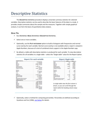
Descriptive Statistics: Tabular and Graphical ent25%20%15%10%5%0%BCSEEHNSMOSBSOSBSBachelor's Degree Field of s Degree Field of Studyc.The lowest percentage for a Bachelor’s is Education (6%) and for Master’s Natural Sciences andMathematics (2%).d.The highest percentage for a Bachelor’s is Other (24%) and for a Master’s is Business (27%).2-7 2018 Cengage. May not be scanned, copied or duplicated, or posted to a publicly accessible website, in whole or in part.
Chapter 's27%9%24%8%2%6%24%Difference6%0%18%-8%-6%-10%- 0%Education has the largest increase in percent: 18%10. a.RatingExcellentVery 649RatingExcellentVery 106100b.c.4540Percent Frequency35302520151050ExcellentVery GoodAveragePoorTerribleRating2-8 2018 Cengage. May not be scanned, copied or duplicated, or posted to a publicly accessible website, in whole or in part.
Descriptive Statistics: Tabular and Graphical Displaysd.29% 39% 68% of the guests at the Sheraton Anaheim Hotel rated the hotel as Excellent or VeryGood. But, 10% 6% 16% of the guests rated the hotel as poor or terrible.e.The percent frequency distribution for Disney’s Grand Californian follows:RatingExcellentVery 6310048% 31% 79% of the guests at the Sheraton Anaheim Hotel rated the hotel as Excellent or VeryGood. And, 6% 3% 9% of the guests rated the hotel as poor or terrible.Compared to ratings of other hotels in the same region, both of these hotels received very favorableratings. But, in comparing the two hotels, guests at Disney’s Grand Californian provided somewhatbetter ratings than guests at the Sheraton Anaheim otalFrequency281110940Relative Frequency0.0500.2000.2750.2500.2251.000Percent Frequency5.020.027.525.022.5100.012.Classless than or equal to 19less than or equal to 29less than or equal to 39less than or equal to 49less than or equal to 59Cumulative Frequency10244148502-9Cumulative Relative Frequency.20.48.82.961.00 2018 Cengage. May not be scanned, copied or duplicated, or posted to a publicly accessible website, in whole or in part.
Chapter -5914. a.6.08.010.012.014.016.0b/c.Class6.0 – 7.98.0 – 9.910.0 – 11.912.0 – 13.914.0 – 15.915.Frequency4283320Percent Frequency2010401515100Leaf Unit .16375 5 781 3 4 893 6100 4 51132 - 10 2018 Cengage. May not be scanned, copied or duplicated, or posted to a publicly accessible website, in whole or in part.
Descriptive Statistics: Tabular and Graphical Displays16.Leaf Unit 10116120 2130 6 7142 2 7155160 2 8170 2 317. a/b.Waiting Time0–45–910 – 1415 – 1920 – 24TotalsFrequency4852120Relative Frequency0.200.400.250.100.051.00c/d.Waiting TimeLess than or equal to 4Less than or equal to 9Less than or equal to 14Less than or equal to 19Less than or equal to 24e.Cumulative Frequency412171920Cumulative Relative Frequency0.200.600.850.951.0012/20 0.6018. 502 - 11 2018 Cengage. May not be scanned, copied or duplicated, or posted to a publicly accessible website, in whole or in part.
Chapter s than 12less than 14less than 16less than 18less than 20less than 22less than 24less than 26less than 28less than 20-2222-2424-2626-2828-30PPGe.There is skewness to the right.f.(11/50)(100) 22%2 - 12 2018 Cengage. May not be scanned, copied or duplicated, or posted to a publicly accessible website, in whole or in part.
Descriptive Statistics: Tabular and Graphical Displays19. a.The largest number of tons is 236.3 million (South Louisiana). The smallest number of tons is 30.2million (Port Arthur).b.Millions Of Histogram for 25 Busiest U.S 4.9 125-149.9 150-174.9 175-199.9 200-224.9 225-249.9Millions of Tons HandledMost of the top 25 ports handle less than 75 million tons. Only five of the 25 ports handle above 75million tons.20. a.Lowest 12, Highest 23b.Hours in Meetingsper 63544252 - 13PercentFrequency4%8%24%12%20%16%16%100% 2018 Cengage. May not be scanned, copied or duplicated, or posted to a publicly accessible website, in whole or in part.
Chapter 2c.76Fequency54321011-1213-14 15-16 17-18 19-20 21-22Hours per Week in Meetings23-24The distribution is slightly skewed to the left.21.a/b/c/d.Visitors uencyCumulative tal501.002 - 14 2018 Cengage. May not be scanned, copied or duplicated, or posted to a publicly accessible website, in whole or in part.
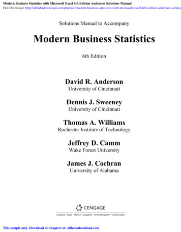
Descriptive Statistics: Tabular and Graphical Displayse.The histogram is highly skewed to the right. Note that there are very few websites that have morethan 100 million visitors.201816Frequency1412108642 0-189190-199200-209210-219220-229230-239240-250 2500Visitors (millions)f.The website with the most U.S. visitors is youtube.com with 222 million U.S. visitors.22. a.# 02 - 15 2018 Cengage. May not be scanned, copied or duplicated, or posted to a publicly accessible website, in whole or in part.
Chapter 2b.1210Frequency86420c.23. a.b.049995000 999910000 1499915000 1999920000 2499925000 29999Number of U.S. Locations30000 3499935000 39999The distribution is skewed to the right. The majority of the franchises in this list have fewer than20,000 locations (50% 15% 15% 80%). McDonald's, Subway and 7-Eleven have the highestnumber of locations.The highest positive YTD % Change for Japan’s Nikkei index with a YTD % Change of 31.4%.A class size of 10 results in 10 classes.YTD % ChangeFrequency-20- -15.11-15- -10.11-10- -5.13-5- 030-34.912 - 16 2018 Cengage. May not be scanned, copied or duplicated, or posted to a publicly accessible website, in whole or in part.
Descriptive Statistics: Tabular and Graphical Displaysc.987Frequency6543210-20- --15- --10- - -5- 0 - 4.9 5 - 9.9 10 15.110.15.10.114.915 19.920 24.925 29.930 34.9YTD % ChangeThe general shape of the distribution is skewed to the left. Twenty two of the 30 indexes have apositive YTD % Change and 13 have a YTD % Change of 10% or more. Eight of the indexes had anegative YTD % Change.d.24.A variety of comparisons are possible depending upon when the study is done.Leaf Unit 1000Starting MedianSalary46851233566011122712588Leaf Unit 1000Mid-Career MedianSalary800493351056611014122366744There is a wider spread in the mid-career median salaries than in the starting median salaries.Also, as expected, the mid-career median salaries are higher that the starting median salaries. Themid-career median salaries were mostly in the 93,000 to 114,000 range while the startingmedian salaries were mostly in the 51,000 to 62,000 range.2 - 17 2018 Cengage. May not be scanned, copied or duplicated, or posted to a publicly accessible website, in whole or in part.
Chapter 225. 100-109 110-119% Increaseb.The histogram is skewed to the right.c.4567891011d.31120033343747695779Rotating the stem-and-leaf display counterclockwise onto its side provides a picture of the data thatis similar to the histogram in shown in part (a). Although the stem-and-leaf display may appear tooffer the same information as a histogram, it has two primary advantages: the stem-and-leaf displayis easier to construct by hand; and the stem-and-leaf display provides more information than thehistogram because the stem-and-leaf shows the actual data.26. a.22334455667b.160506051624716060641737071 2 373 3 3 3 4 492 29Most frequent age group: 40-44 with 9 runners2 - 18 2018 Cengage. May not be scanned, copied or duplicated, or posted to a publicly accessible website, in whole or in part.
Descriptive Statistics: Tabular and Graphical Displaysc.43 was the most frequent age with 5 runners27. 27.80.0B61.116.7C11.183.3Total100.0100.0Category A values for x are always associated with category 1 values for y. Category B values for xare usually associated with category 1 values for y. Category C values for x are usually associatedwith category 2 values for y.2 - 19 2018 Cengage. May not be scanned, copied or duplicated, or posted to a publicly accessible website, in whole or in part.
Chapter 228. a.20-39x10-2930-4950-6970-90Grand Total21473y60-791413640-5980-1004Grand 00y60-7916.766.716.70.010080-10080.0Grand 30-4950-6970-90Grand Total80-100100.00.0
The purpose of Modern Business Statistics is to provide students, primarily in the fields of business administration and economics, with a sound conceptual introduction to the field of statistics and its many applications. The text is applications-oriented and has been written with the needs of the nonmathematician in mind.