Transcription
Statistical Energy Analysis softwareDevelopment and implementation of an open source codein Matlab/OctaveMaster’s Thesis in the Master’s programme in Sound and VibrationDANIEL JOHANSSONPETER COMNELLDepartment of Civil and Environmental EngineeringDivision of Applied AcousticsVibroacoustics GroupCHALMERS UNIVERSITY OF TECHNOLOGYGöteborg, Sweden 2010Master’s Thesis 2010:130
MASTER’S THESIS 2010:130Statistical Energy Analysis softwareDevelopment and implementation of an open source code in Matlab/OctaveMaster’s Thesis in the Master’s programme in Sound and VibrationDANIEL JOHANSSONPETER COMNELLDepartment of Civil and Environmental EngineeringDivision of Applied AcousticsVibroacoustics GroupCHALMERS UNIVERSITY OF TECHNOLOGYGöteborg, Sweden 2010
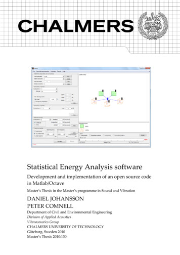
Statistical Energy Analysis softwareDevelopment and implementation of an open source code in Matlab/OctaveMaster’s Thesis in the Master’s programme in Sound and VibrationDANIEL JOHANSSONPETER COMNELL DANIEL JOHANSSON, PETER COMNELL 2010Master’s Thesis 2010:Department of Civil and Environmental EngineeringDivision of Applied AcousticsVibroacoustics GroupChalmers University of TechnologySE-412 96 GöteborgSwedenTelephone: 46 (0)31-772 1000Cover:Graphical user interface of the developed software, SEAlab, demonstrating aSEA model of a double leaf wall.
Chalmers reproserviceGöteborg, Sweden 2010
Statistical Energy Analysis softwareDevelopment and implementation of an open source code in Matlab/OctaveMaster’s Thesis in the Master’s programme in Sound and VibrationDANIEL JOHANSSON & PETER COMNELLDepartment of Civil and Environmental EngineeringDivision of Applied AcousticsVibroacoustics GroupChalmers University of TechnologyABSTRACTThe available software for calculating Statistical Energy Analysis (SEA) isoften written with closed source code. A user defines some input data for asystem and will be presented with a result but with no information on howthese results were calculated. The software acts like a “black box”. There areusually also limited possibilities to modify specific alterations to thesecalculations. Therefore there is a need for software that is written in opensource code which gives the user possibilities to modify calculation methodsand provide a better understanding on how to interpret the results.Another problem with today’s SEA-calculation software are that they areoften combined with other software into large packages which makes themquite expensive and may force the users to purchase software that are of nouse for them. With open source code, the software will always be free ofcharge and available for anyone to use.The aim of this Master s Thesis has been to construct a SEA-calculationsoftware using open source code in Matlab, with the key component to designit in such a way that future developments can easily be made.Focus in this thesis has been on implementing SEA-calculation methods forsystems build up of isotropic plates connected via a line junction. Areaconnections are also implemented in order to calculate the soundtransmission between rooms separated by single or double leaf walls. Themethod used to make this possible has been literature study and MATLABprogramming.Validations of the results are carried out by comparing three examples to ascientific article and a commercial software called AutoSEA v.1.5. The threeexamples are; two plates coupled together over a line junction, soundtransmission through a single leaf wall and sound transmission through adouble leaf wall.Conclusions of the work is that the results correlates well with the article andthe commercial software with the exception of the non-resonant transmissionof the double leaf wall which needs to be further evaluated and validated.Key words: statistical energy analysis, SEA, coupling loss factor, modaloverlap, modal density, transmission coefficient, radiation efficiency, opensource codeI
II
N11.1Background11.2Aim11.3Goal12SOFTWARE SOURCE CODE23THEORY OF STATISTICAL ENERGY ANALYSIS3453.1System definition43.2General SEA equations53.3Input power73.4Energy93.5Damping93.6Coupling loss factor113.7Modal density143.8Modal overlap153.9SEA assumptions and restrictions3.9.1Energy flow and modal energies3.9.2Strong and weak coupling3.9.3Modal overlap and number of modes3.9.4Uncorrelated sources3.9.5Conservative coupling3.9.6Maximum length3.9.7Maximum height16161617181818183.1019Material propertiesCLF-COEFFICIENTS CALCULATION204.1Transmission coefficients204.2Radiation efficiency from finite plates274.3Non-resonant transmission29VALIDATION5.1Structural transmission coefficients3131
5.2Single leaf wall405.3Double leaf wall example456DISCUSSION517CONCLUSION547.18Further workREFERENCES5556APPENDIX A – DATA AND FOLDER STRUCTURE57APPENDIX B – USER GUIDE71II
PrefaceThis thesis work has been carried out during spring and autumn of 2010 as apart of the finalization of the masters program at the Division of AppliedAcoustics at the Chalmers University of technology in Gothenburg, Sweden.The basis of this work mostly consists of literature study and programming inMatlab.We would like to take the opportunity to thank the people who in some waycontributed to the work.First of all we would like to thank our supervisor at Chalmers; PatrikAndersson for his useful input and willingness to help us. We would also liketo thank our supervisors from A2Zound; Lars Ivarsson and Henrik Marbergfor their constructive input and discussion of the software layout andhandling and a special thanks to Lars whose idea it was to start this project.The willingness of Jens Forssén to take the time to answer our questions hasbeen much appreciated. Also the technical help from Börje Wijk was of highvalue to us and saved us a lot of time.Göteborg September 2010Daniel JohanssonPeter Comnell
NotationsRoman upper case letters Total absorptionBending stiffness Energy Spring stiffness of cavity (N/m) ′Young s modulusForce (N)Length of the line connection (m)Length of perimeter (m)Traction force according to Figure 4.2Traction force according to Figure 4.2Power Volume velocity (m3/s) ′Surface area (m2) Reduction indexRadiation resistance Surface area of a volume (m2) Traction force according to Figure 4.2 Traction force according to Figure 4.2Reverberation time (s)Volume (m3)MobilityImpedanceRoman lower case letters Wave speed in fluid (m/s)Group speed (m/s)Cavity width (m) First mode shape (Hz)IVFrequency (Hz)Critical frequency (Hz)Double leaf wall resonance frequency (Hz)
Cavity stops acting like a spring with constant stiffness (Hz)ℎ!Height (m)%&Mass (kg)Wave number"Length (m), " " 'Modal density(Pressure (Pa)* Velocity (m/s)) * Time (s)Displacement according to Figure 4.2Displacement according to Figure 4.2Displacement according to Figure 4.2Greek lower case letters,,′Wave amplitude-.Total loss factor for subsystem 0.2 Plate-Plate junction angleAbsorption coefficient-Loss factor-. Internal loss factor for subsystem 0.-./23Coupling loss factor, from subsystem 0 to 1.Displacement according to Figure 4.24Poissons ration.6Density of fluid (kg/m3)55 789Wave length (m)2Mass per unit area (kg/m )Radiation efficiencyTransmission coefficientIncident wave angleAngular frequency
Vectors & Matrixes:; ?Dynamic stiffness matrixGeometrical matrixForce vectorDisplacement vectorDisplacement vectorDynamic load vectorAcronymsCLFCoupling Loss FactorSEAStatistical Energy AnalysisVI
1 IntroductionStatistical energy analysis has been used as an estimation technique for midand high frequency vibration and sound transmission since it first arose in themid 1960 s. SEA, short for Statistical energy analysis, has since then provensuccessful and has today a wide application range, stretching from buildingsto spacecraft.1.1 BackgroundThe available software for calculating SEA often has closed source code whichmeans that the user does not know how the software calculates the results, thesoftware acts like a “black box” e.g. the user loads input data and the softwarereturns results and everything in-between remains hidden from the user.Another incitement for this thesis is that the commercial SEA software is oftencombined with other software into larger packages. The license for such apackage is often expensive and may come with software that are of no use tothe user.1.2 AimThe aim of this master thesis is to construct and implement an SEAcalculation software. The software, called SEAlab, should be written in Matlaband the programming should be well documented and open for the user.SEAlab should be designed in such a way that future modifications couldeasily be made. As a start the software should be able to handle isotropic platetransmission and sound transmission between rooms separated by a wallconstructed by single or double leafs.1.3 GoalThe goal is to construct a user-friendly Matlab program that conducts SEAcalculations. The software should be constructed in such a way that it couldeasily be modified to the user’s specifications. This will be fulfilled by the useof functions in the program. Functions can easily be overviewed andmodified. The use of functions enables the user to create new function thatcan be integrated in the software.CHALMERS, Civil and Environmental Engineering, Master’s Thesis 2010:1301
2 Software source codeAll software has a source code. Usually the source code is open or closed tothe user, meaning if the user has access to the source code or not. There aremany different types of licenses that regulate the user insight andmodification capabilities in the software. The source code in SEAlab is openfor everyone and is regulated by the BSD license: [11]Copyright (c) 2010, Daniel Johansson & Peter ComnellAll rights reserved. Redistribution and use in source and binary forms, with or withoutmodification, are permitted provided that the following conditions aremet:Redistributions of source code must retain the above copyright notice,this list of conditions and the following disclaimer.Redistributions in binary form must reproduce the above copyrightnotice, this list of conditions and the following disclaimer in thedocumentation and/or other materials provided with the distribution.Neither the name of the technical university of Chalmers, Gothenburgnor the names of its contributors may be used to endorse or promoteproducts derived from this software without specific prior writtenpermission.THIS SOFTWARE IS PROVIDED BY THE COPYRIGHT HOLDERS ANDCONTRIBUTORS "AS IS" AND ANY EXPRESS OR IMPLIED WARRANTIES,INCLUDING, BUT NOT LIMITED TO, THE IMPLIED WARRANTIES OFMERCHANTABILITY AND FITNESS FOR A PARTICULAR PURPOSE AREDISCLAIMED. IN NO EVENT SHALL THE COPYRIGHT HOLDER ORCONTRIBUTORS BE LIABLE FOR ANY DIRECT, INDIRECT, INCIDENTAL,SPECIAL, EXEMPLARY, OR CONSEQUENTIAL DAMAGES (INCLUDING,BUT NOT LIMITED TO, PROCUREMENT OF SUBSTITUTE GOODS ORSERVICES; LOSS OF USE, DATA, OR PROFITS; OR BUSINESSINTERRUPTION) HOWEVER CAUSED AND ON ANY THEORY OFLIABILITY, WHETHER IN CONTRACT, STRICT LIABILITY, OR TORT(INCLUDING NEGLIGENCE OR OTHERWISE) ARISING IN ANY WAYOUT OF THE USE OF THIS SOFTWARE, EVEN IF ADVISED OF THEPOSSIBILITY OF SUCH DAMAGE.The advantage with an open source code is that the user can inspect the codeand see exactly how the software processes the input data. Open source alsomakes it easier for the user to modify and create own applications to thesoftware according to his/hers specifications.Matlab were chosen as the programming language because it is widely usedand it is relatively cheap in comparison to SEA software. Also it is closelyrelated to the free software Octave. Many of the important functions used inSEAlab works in an Octave environment.2CHALMERS, Civil and Environmental Engineering, Master’s Thesis 2010:130
3 Theory of Statistical Energy AnalysisStatistical Energy Analysis, or (SEA) is a structural-acoustic method that iswidely used. SEA arose during the 1960 s in the aerospace industry to predictthe vibrational behavior when designing space craft. During this timecomputational methods were available but the size of the models that couldbe handled and the computational speed were such that only few of thelowest order modes could be predicted. [1] Furthermore, in traditionalanalysis of mechanical vibration the lowest modes are usually of most interestbecause these modes normally have the greatest displacement response. Butwhen designing and constructing large and lightweight aerospace structuresit is apparent that also high frequency broad-band loads is important in theprocess of predicting structural fatigue, equipment failure and noiseproduction. [2] The development and use of SEA proved to be a good methodto predict high frequency loads and the analysis technique has since then beenapplied, extended and developed for a growing number of applications. Forexample it has been used to model sound and vibration transmission inbuildings, cars, aircrafts, ships and trains. [3]The name SEA points out certain aspects of the method. Statistical accents thatthe system being considered are a member of a population of similar systemswith known distributions of the subsystem parameters. Energy is the variableof interest. It describes the behavior of the system in terms of stored,dissipated and exchanged energies of vibration. Other often used variables foracoustic and structural vibration, such as displacement, pressure etc. can bederived from the energy of vibration. Analysis emphasizes that SEA is aframework rather than a specific technique. [2]In order to model the exchange of vibrational energy within a system, it iscrucial that the system is divided into several subsystems. SEA models thesound transmission in systems and energy distribution over the subsystemsby power balance equations. Total incoming power on one hand and the totaldissipated power on the other are equal.In order to evaluate how the transferred power between the subsystems arerelated to their equilibrium energies, certain transmission coefficients needs tobe evaluated. There are three main approaches to estimates these coefficients.These are the modal approach, the wave approach and the mobility approach.The modal approach governs the interaction of the uncoupled modes in thesubsystems. With boundary conditions which express the decoupling it ispossible to express the multimode power transfer coefficients. This approachis well suited for vibroacoustic problems involving acoustic interactionbetween enclosed volumes. The modal approach is not ideally suited tocouplings between solid structures, this is where the second approach comesin handy, the wave approach. In this approach the vibrational fields aremodeled as superposition of traveling waves and the transferred powerbetween subsystems can be derived from wave transmission and reflections atthe subsystem interfaces. The third approach is the mobility approach.CHALMERS, Civil and Environmental Engineering, Master’s Thesis 2010:1303
The mobility approach utilizes the concept of dynamic mobility, or impedanceto express the interaction of the coupled subsystems.[1]In this project the wave approach is utilized for coupling between structures,for couplings with volumes a standardized method reference [4] will beutilized. The main reason for this method is that it is commonly used amongengineers and that it is a standardized method.3.1 System definitionSound transmission through for example a wall in a building is onlyrepresented by a limited part of the entire building, ‘the system’. It isimportant that the model contain as much as possible of the influencing partsof the building to provide reliable results. However, not more than necessaryshould be treated in order to not make it to complex which increases thechance of errors and also larger computation times.In SEA, each system is divided into several physical elements of a suitablesize. These elements are divided so that the vibro-acoustic characteristics aresimilar over them, such as damping, excitation and coupling properties. Theseelements are called subsystems. For example, an isotropic plate is usuallytreated as three subsystems corresponding to the different wave types in theplate, (flexural, longitudinal and shear waves). Only wave types that play animportant part in the transmission, dissipation and storage of energy need tobe included as subsystems in a model. So for example in a fluid volume onlylongitudinal waves are important for the sound transmission and the fluidvolume can therefore be treated as a single subsystem.4CHALMERS, Civil and Environmental Engineering, Master’s Thesis 2010:130
3.2 General SEA equationsThe principles of SEA can be illustrated as shown in Figure 3.1 below. Thissystem consists of two connected subsystems.Figure 3.1 SEA model of two subsystems.Energy flows in and out of a subsystem. The energy that flows out consist ofdissipation ( . and / ), radiation and transmission to other subsystems ( ./or /. ). The energy that flows into a subsystem consist of external sourceexcitations ( . and / ) and transmissions from other subsystems ( ./ or /. ).The dissipated power in a subsystem is given by equation 3.1 below:. 9-. .(3.1)where -. is referred to as the damping loss factor and . is the totalvibrational energy of the modes at frequency .The net transmitted power between subsystem i and j (equation 3.2./ 9-./ ./ )is given by(3.2)SEA calculation is based on energy flow equilibrium. The power balances forthe two systems are given as in equations 3.3 and 3.4./ /./ .//. . / CHALMERS, Civil and Environmental Engineering, Master’s Thesis 2010:130(3.3)(3.4)5
When combining equations 3.1-3.4, the power balance equation for twosubsystems can be expressed in matrix form shown in equation 3.5B C 9D./E-. -./ F -./ -/. .H B C(3.5) . -L. / M JM -L L(3.6)E-/ -/. F/For a more generalized case with & number of subsystems, the balanceequations can be written in a general form as, equation 3.6-. ./J /M 9 J -.LL -/.-/ . Where -. equals the total loss factor and is the summation of the damping lossfactor of the subsystem and the coupling loss factors representing energytransmission from the subsystem to others, equation 3.7.nηi ηid η(3.7)ijj 1, j iThe matrix can also be described in a symmetric form as in equation 3.8.-. &. -./ &.J /M 9 J .L &.L. -/. &/-/ &/ . /&. -L. &L / /&/ M J M-L &L L /&L(3.8)Where & is the modal density, further described in chapter 3.9. The generalmatrix and the symmetric is basically the same except that the energy is nowdescribed as the modal energy instead of energy as in the general matrix. Themodal energy is defined as the energy in the subsystem divided by the modaldensity. The advantage of describing the matrix in a symmetric form is thatthe consistency relationship can be used. The consistency relationship statesthe relation between two subsystems modal energies and their coupling lossfactors as shown in equation 3.9.&. -./ &/ -/.6(3.9)CHALMERS, Civil and Environmental Engineering, Master’s Thesis 2010:130
By using the consistency relationship only the coupling loss factors for onetransmission direction are needed to calculate the energy exchange betweentwo subsystems. This means that only the upper triangular or the lowertriangular side of the symmetric matrix explained in equation 3.8 needs to becalculated, the rest can be calculated by the consistency relationship andthereby save a lot of numerical calculations. [3]For most systems, especially large systems, many subsystems are notconnected. This means that the matrix will contain many zero off-diagonalelements and therefore a sparse matrix. If the consistency relationship isapplied, prediction tools can utilize this to lower the computation time andrequired memory usage. For SEA modeling these matrixes will for mostsystems still be relatively small compared to for example those used in FEMmodels and given the performance of today’s computers, using theconsistency relationship, will not greatly affect the calculation speed. Forsome systems that require much computation performance, the consistencyrelationship should if possibly still be used. An example of this is platescoupled over a line junction at a certain connection angle and averaged overmany incident angles to create a diffuse sound field in the plate, this will bedescribed in chapter 3.3.3 Input powerThere are different ways to excite the structure and depending on the sourcethe energy input in the subsystem differs. The different types of input powercan for example be: mechanical point excitation or an acoustic source.These external sources inject energy into one or more subsystems of a system.These sources can be described as forces, moments, pressures or motions.The mechanical point excitations can be described as a force source or velocitysource as:Force source:. (S) U ℜWX(S)Y (3.10)Velocity source:. Z[(S)U ZℜW\(S)Y (3.11)where is the force, * is the velocity and ℜW Y is the real part of the pointmobility and ℜW Y is the real part of the impedance.CHALMERS, Civil and Environmental Engineering, Master’s Thesis 2010:1307
The force and velocity * are related by the point mobility and impedanceaccording to:* (3.12) *(3.13)Depending on the excitation point the real part of the mobility can becalculated for a plate by the equations shown in the table below.ℜW Y18 513.5 5 29 ℎTable 3.1 Different types of point excitations and their corresponding real part of the mobilitywhere is the bending stiffness of a plate, 5 the mass per unit area, theYoung’s modulus and ℎ the thickness of the plate.Acoustic sources usually have constant velocity, not constant power. Theradiated power can be calculated by the equation. eeee (3.14)eeee is the mean-square volume velocity and is the radiation resistanceand can be calculated for a point source in free field as: 8fg h igUjk(3.15)CHALMERS, Civil and Environmental Engineering, Master’s Thesis 2010:130
where 5 , and ! are the density, wave speed and wave number in the freefield respectively. [5]3.4 EnergyAs mentioned earlier the vibrational energy is the primary response variableof subsystems and it can be expressed in other acoustic variables that is morecommon, such as pressure and velocity.For an acoustic subsystem 0 the energy is given by: . lmU nmfm mU(3.16)'. is the sound pressure (r.m.s.) averaged over the acoustic volume . . 5. and . are the density and the wave speed in the medium.For a structural subsystem the Energy is given by: . %. *. (3.17)where *. is the velocity (r.m.s.) averaged over the surface area and %. the totalmass of the subsystem.3.5 DampingThe damping loss factor of a subsystem can be described as:-., -.,p -., -.,q(3.18)where:-.,p is the loss factor for structural or material damping in the subsystem. Thisis basically the conversion from vibrations into heat.-., is the loss factor associated with acoustic radiation losses from thesurface of the subsystem into the surrounding fluid medium. This can also beexplained as the conversion of vibrations into sound. If the surroundingmedium however is modeled as a subsystem in the system with its respectivetransmission coupling loss factor, this loss factor is not taken into account inthe damping loss factor of subsystem 0. The sound level caused in the roomcan then be predicted instead of just being included in the damping lossfactor.CHALMERS, Civil and Environmental Engineering, Master’s Thesis 2010:1309
-.,q is the loss factor associated with coupling damping for subsystem 0. Thiscontribution can often be neglected in SEA modeling due to the assumptionmade that no energy is lost in the coupling. [12]As mentioned before from equation 3.7 the total loss factor -. can be describedas the sum of all coupling loss factors from the subsystem to the otherconnected subsystems and the damping loss factor -., for the subsystem. Thistotal loss factor is sometimes described to as the subsystem’s damping.There are several ways to estimate the total loss factor -. for different types ofsubsystems without the need to calculate the damping loss factor or all thecoupling loss factors to connecting subsystems. In building acoustics the mostcommon way to calculate the total loss factor for a room is to use thereverberation time. The equation used to calculate the total loss factor thenbecomes:-. rs . tg(3.19)Where is the reverberation time and is defined as the time it takes for theenergy to decrease with 60dB from a steady state condition. The formula canbe used for rooms as well as for structures but it can be difficult to measurethe reverberation time in structures because of the short reverberation time.Large structures, like buildings, can be challenging to excite sufficiently.The reverberation time can be calculated in rooms if the absorption of theroom is known. . nu(3.20)Where A is the total absorption in a room and can be calculated as ,′(3.21)Here is the surface area that is multiplied with its corresponding absorptioncoefficient ,′.To estimate the total loss factor for a room when the reverberation time isunknown, a typical absorption of 10% or a reverberation time of 0.5seconds can be used. [3]10CHALMERS, Civil and Environmental Engineering, Master’s Thesis 2010:130
When calculating the total loss factor for a cavity, as can be seen in doublewalls, the total loss is estimated by a different equation.-. g xyz kr{(3.22)Where " is the length multiplied with its corresponding absorption coefficient,′. A cavity is here defined as a room were the wave propagation is 2dimensional. It is important to keep in mind that the value of the absorptioncoefficient ,′ differs if a material is placed in a cavity or a room. [3]3.6 Coupling loss factorThe coupling loss factor is a parameter that is uniquely associated with SEA.It is possible to relate the coupling loss factors to other parameters that areused outside SEA such as radiation efficiency and transmission coefficients,which will be seen in the following equations in this chapter.Coupling loss factors are used in SEA to describe the energy transmitted fromone subsystem to another. The equations differ depending on the type ofjunction and the properties of the connected subsystems. The formulaspresented below is the formulas used in the software and can be found inliterature.The coupling loss factor is defined as the fraction of energy that transmitsfrom one subsystem to another. As described before the power transmittedfrom subsystem 1 to subsystem 2 for a general case can be described as: 9- (3.23)The energy in subsystem 1 can be described as mentioned before as: % * (3.24) 5 * (3.25)Where % is the mass and * is the rms and spatial average of the velocity insubsystem 1. For a 2-dimensional subsystem, plates and cavities, equation3.24 can be written as:5 and are the density and surface area of subsystem 1. For a 3-dimensionalsubsystem, rooms, equation 3.24 can be described as:CHALMERS, Civil and Environmental Engineering, Master’s Thesis 2010:13011
5 * (3.26)Where 5 is the fluid density and is the volume. Combining equations 3.23and 3.25 provides the following expression for a 2-dimensional case. 5 * 9- (3.27)For two coupled plates the power transmission between the two plates can bedescribed as Lp .L 7(3.28)Where 7 is the transmission coefficient. Using the properties of a 2dimensional diffuse field the incoming power can be described as.L } k{ f [ U k(3.29)Here is the length of the conncetion. Combining equations 3.27-3.29, thecoupling loss factor for a plate-plate model can be described as:- USk{ (3.30)Where 7 is the transmission coefficient between subsystem 1 and 2. is thegroup speed and is calculated by the following equations for bending,longitudinal and shear waves. For bending waves the group speed is twicethe phase speed q and is calculated as: ,q 2 q 2 S Uf j(3.31)where is the bending stiffness of the plate: 12} ( U )(3.32)CHALMERS, Civil and Environmental Engineering, Master’s Thesis 2010:130
is the Young’s modulus, ℎ is the thickness of the plate and 3 is Poisson’sratio. For longitudinal and shear waves, the group speed is equal to the wavespeed: ,x x } f( U )(3.33) ,p p f( )} (3.34)When coupling a plate and a room, the coupling loss factor can be calculatedin a similar way as for coupling two plates. Here the radiated power isdefined as a fraction of the incoming wave as lx L 6Where 6 is the radiation efficiency andsurface generating a plane wavelx L (3.35)lx L is the radiated power of a flat * 5 (3.36)5 , and are the mass per unit area, speed of sound and surface area. Bysetting equation 3.27 as the radiated power and combining it with equations3.35-3.36 above one obtains- fg g Sf (3.37)The non-resonant coupling loss factor for a room to another room or from aroom to a cavity is defined as equation 3.28 but now the incoming power isdescribed as.L } g { jn (3.38) is the volume. Similar to coupling between two plates, equation 3.28 arecombined with equation 3.38 and equation 3.26 to describe the coupling lossfactor for room to room or room to cavity as:CHALMERS, Civil and Environmental Engineering, Master’s Thesis 2010:13013
- g { UjSn (3.39)The consistency relation, equation 3.9, is used with equation 3.39 to calculatethe coupling loss factor from a cavity to a room.3.7 Modal densityModes is an essential part of SEA and occurs when the multiple of thewavelength of a subsystem and the dimensions of the subsystem match.When this happens the amplitude becomes larger due to constructiveinterference between waves travelling in the subsystem. Modes can also bereferred to as resonances. The m
Statistical Energy Analysis software Development and implementation of an open source code in Matlab/Octave Master’s Thesis in the Master’s programme in Sound and Vibration DANIEL JOHANSSON PETER COMNELL Department of Civil an
