Transcription
The Finite Element Method – Lecture NotesPer-Olof Perssonpersson@berkeley.eduMarch 10, 202211.1Introduction to FEMA simple exampleConsider the model problem u00 (x) 1, for x (0, 1)u(0) u(1) 0(1.1)(1.2)with exact solution u(x) x(1 x)/2. Find an approximate solution of the formû(x) A sin(πx) Aϕ(x)(1.3)Various ways to impose the equation:Collocation : Impose û00 (xc ) 1 for some collocation point xc Aπ 2 sin(πxc ) 1 xc xc 1214 A A 1 0.1013π2 2 0.1433π2Average : Impose the average of the equation over the interval:Z 1Z 100 û (x) dx 1 dx00Z 12Aπ 2 sin(πx) dx Aπ 2 2Aπ 1π01A 0.1592πGalerkin : Impose the weighted average of the equation over the interval:Z 1Z 100 û (x)v(x) dx 1 · v(x) dx0(1.4)(1.5)(1.6)(1.7)0A Galerkin method using the weight functions v(x) from the same space as the solutionspace, that is, v(x) ϕ(x). This givesZ 1Z 1Aπ 2 sin2 (πx) dx sin(πx) dx(1.8)0012Aπ · 2π4A 3 0.129π21(1.9)(1.10)
0.180.16ûAVG (x)0.14ûGAL (x)0.12u(x)0.10ûCOL (x)0.080.060.040.020.000.00.20.40.60.81.0Figure 1: Solutions of the model problem (1.1)-(1.2) using collocation, average, andGalerkin.The three solutions are shown in figure 1.1. The finite element method is based on theGalerkin formulation, which in this example clearly is superior to collocation or averaging.1.2Other function spacesUse piecewise linear, continuous functions of the form û(x) Aϕ(x) with(2xx 21ϕ(x) 2 2x x 12Galerkin gives the FEM formulationZ 1Z û00 (x)ϕ(x) dx 0(1.11)1ϕ(x) dx(1.12)0Since û00 is not bounded, integrate LHS by parts:Z 1Z 1 0 100û (x)ϕ (x) dx û (x)ϕ(x) 0 û0 (x)ϕ0 (x) dx û0 (1)ϕ(1) û0 (0)ϕ(0)00Z 1 û0 (x)ϕ0 (x) dx,(1.13)(1.14)0since ϕ(0) ϕ(1) 0. This leads to the final formulationZ 1Z 100û (x)ϕ (x) dx ϕ(x) dx.0(1.15)0To solve for û(x) Aϕ(x), note that û0 (x) Aϕ0 (x) and(2x 12ϕ0 (x) 2 x 122(1.16)
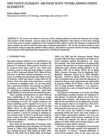
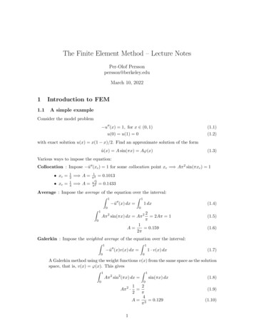
u3u1u2ϕ2ϕ11x0x1ϕ3x2x3x4Figure 2: A refined piecewise linear function space, same solution and basis functions.Equation (1.15) then becomesZ 1/2Z 1Z(2A)(2) dx ( 2A)( 2) dx 01/21/2Z12x dx 0(2 2x) dx(1.17)1/2or 4A 1/2, that is, A 1/8, and the FEM solution is û(x) ϕ(x)/8.1.3More basis functionsTo refine the solution space, introduce a triangulation of the domain Ω [0, 1] into nonoverlapping elements:Th {K1 , K2 , . . .}(1.18)such that Ω K Th K. Now consider the space of continuous functions that are piecewiselinear on the triangulation and zero at the end points:Vh {v C 0 ([0, 1]) : v K P1 (K) K Th , v(0) v(1) 0}.(1.19)Here Pp (K) is the space of polynomials on K of degree at most p. Define a basis {ϕi } forVh by the basis functions ϕi Vh with ϕi (xj ) δij , for i, j 1, . . . , n. Our approximatesolution uh (x) can then be written in terms of its expansion coefficients and the basisfunctions asuh (x) nXui ϕi (x),(1.20)i 1where we note that this particular basis has the convenient property that uh (xj ) uj , forj 1, . . . , n.A Galerkin formulation for (1.1)-(1.2) can now be stated as: Find uh Vh such thatZ 1Z 100uh (x)v (x) dx v(x) dx, v Vh(1.21)003
In particular, (1.21) should be satisfied for v ϕi , i 1, . . . , n, which leads to n equationsof the formZ 1Z 100uh (x)ϕi (x) dx ϕi (x) dx,for i 1, . . . , n(1.22)00Insert the expression (1.20) for the approximate solution and its derivative, u0h (x) Z 1 XZ 1n00 uj ϕj (x) ϕi (x) dx ϕx (x) dx,i 1, . . . , n00i 1 ui ϕi (x):(1.23)0j 1Change order of integration/summation: Z 1 ZnX00ϕi (x)ϕj (x) dx ujj 1Pn1ϕi (x) dx,i 1, . . . , n(1.24)00This is a linear system of equations Au f , with A [aij ], u [ui ], f [fi ], fori, j 1, . . . , n, whereZ 1aij ϕ0i (x)ϕ0j (x) dx(1.25)0Z 1fi ϕi (x) dx(1.26)0Example : Consider a triangulation of [0, 1] into four elements of width h 1/4 betweenthe node points xi ih, i 0, . . . , 4. We then get a solution space of dimensionn 3, and basis functions ϕ1 , ϕ2 , ϕ3 . When calculating the entries of A, note that A is symmetric, that is, aij aji A is tridiagonal, that is, aij 0 whenever i j 1 For our equidistant triangulation, aii ajj and ai,i 1 aj,j 1This gives11 ( 4)( 4) 8441 ( 4) · 4 · 44 a33 a11 8a11 4 · 4 ·(1.27)a12(1.28)a22(1.29)a21 a12 a23 a32 4(1.30)a13 a31 0(1.31)andZf1 f2 f3 1ϕ1 (x) dx 014and the linear system becomes 8 4 0u11/4 4 8 4 u2 1/4 0 4 8u31/44(1.32)(1.33)
with solutionu (u1 , u2 , u3 )T (3/32, 1/8, 3/32)T(1.34)Note that the discretization exactly matches the one obtained with finite differencesand the 2nd order 3-point stencil: 12 1 0u11 1 2 1u2 1 (1.35)(1/4)210 1 2u31.4Neumann boundary conditionsThe Dirichlet conditions u(0) u(1) 0 where enforced directly into the approximationspace Vh . In the finite element method, a Neumann condition (or natural condition) isinstead implemented by modifying the variational formulation. Consider the model problem u00 (x) f (x) for x (0, 1)(1.36)u(0) 0(1.37)0u (1) g(1.38)The function space is only enforcing the Dirichlet condition at the left end point:Vh {v C 0 ([0, 1]) : v K P1 (K) K Th , v(0) 0},(1.39)which in our example gives an additional degree of freedom. The Neumann conditionappears in the formulation after integration by parts:Z 1Z 1 1û0 (x)v 0 (x) dx û0 (1)v(1) û0 (0)v(0)(1.40)û0 (x)v 0 (x) dx û0 (x)v(x) 0 00Z 1 û0 (x)v 0 (x) dx gv(1)(1.41)since v(0) 000and uh (1) g. This leads to the final formulation:Z 1Z 100f (x)v(x) dx gv(1),uh (x)v (x) dx 00Find uh Vh such that v Vh(1.42)Example : With our previous triangulation, we now get another basis function ϕ4 . Forsimplicity, set f g 1. All the matrix entries and right-hand side values are thenidentical, and we only calculate the new values:1a44 (4)2 4(1.43)41a34 a43 ( 4) · 4 · 4(1.44)419f4 g · 1 (1.45)88The linear system then becomes 8 4 00u11/4 4 8 4 0 u2 1/4 (1.46) 0 4 8 4 u3 1/4 00 4 4u49/8with solutionu (u1 , u2 , u3 , u4 )T (15/32, 7/8, 39/32, 3/2)T .5(1.47)
1.5Inhomogeneous Dirichlet problemsUse two spaces: Vh , which enforces the inhomogeneous Dirichlet condition, for the solution uh , and Vh0 , which enforces homogeneous Dirichlet conditions, for the test function v.Consider for example the model problem u00 (x) f, for x (0, 1)(1.48)u(0) 0(1.49)u(1) 1(1.50)with exact solution u(x) x(3 x)/2. Use the spacesVh {v C 0 ([0, 1]) : v K P1 (K) K Th , v(0) 0, v(1) 1},(1.51)Vh0(1.52)0 {v C ([0, 1]) : v K P1 (K) K Th , v(0) 0, v(1) 0}.The FEM formulation becomes: Find uh Vh such thatZ 1Z 10 0f v dx, v Vh0 .uh v dx (1.53)00Note that the function space Vh is not a linear vector space, due to the inhomogeneousconstraint. In practice, Dirichlet conditions are implemented by first considering the allNeumann problem, and enforcing the Dirichlet conditions directly into the resulting systemof equations.Example : For the model problem (1.48)-(1.50), first consider the corresponding allNeumann problem u00 (x) f, for x (0, 1)00u (0) u (1) 0(1.54)(1.55)with the solution spaceVh {v C 0 ([0, 1]) : v K P1 (K) K Th }.(1.56)In our example with four elements of size h 1/4, this gives 5 degrees of freedom andthe resulting linear system (with f 1): 1/84 4 000u1 4 8 4 0 0 u2 1/4 0 4 8 4 0 u3 1/4 (1.57) 00 4 8 4 u4 1/4 1/8u5000 4 4This system is singular (since the solution is undetermined up to a constant). We cannow impose the Dirichlet conditions u(0) 0 and u(1) 1 directly by replacing thecorresponding equations: 10000u10 4 8 4 0 0 u2 1/4 0 4 8 4 0 u3 1/4 (1.58) 00 4 8 4 u4 1/4 00001u516
We can keep the symmetry of the matrix by eliminating the entries below/above thediagonal of the Dirichlet variables: 00u11 000 0 0 8 4 0 0 u2 1/4 ( 4) · 0 1/4 1/4 0 4 8 4 0 u3 1/4(1.59) 0 0 4 8 0 u4 1/4 ( 4) · 1 17/4 11u50 000 1with solution u (u1 , . . . , u5 )T (0, 11/32, 5/8, 27/32, 1)T . If necessary, the Dirichletdegress of freedom can be removed from the system, to obtain the smaller system ofequations 8 4 0u21/4 4 8 4 u3 1/4 (1.60)0 4 8u417/41.6The stamping method (“Assembly”)Consider a single element ek , and its local basis functions Hik (x), j 1, 2, given by therestriction of the global basis functions ϕj (x) to the element. The connection between thelocal indices i and the global indices j are given by a mesh representation. For simplexelements, we use the form p: N D node coordinates t: T (D 1) element indicesHere, row k of t is the local-to-global mapping for element k. The local basis functions are: Defined only inside the element ek Polynomials of degree 1We can then define an elemental matrix Ak , or a local stiffness matrix, by again consideringonly the contribution to the global stiffmatrix from element ek :ZkAij (Hik )0 · (Hjk )0 dx,i 1, 2, j 1, 2(1.61)ekand, similarily, an elemental load vector bk byZkbi f (x) · (Hik ) dx,i 1, 2(1.62)ekIn the so-called stamping method, or the assembly process, each element matrix andload vector are added at the corresponding global position in the global stiffness matrix andright-hand side vector:A 0, b 0for all elements kCalculate Ak , bkA(t(k, :), t(k, :)) Akb(t(k, :)) bkend for7
Example : Equidistant 1D mesh, element width h, piece-wise linears, f 1. The elementalmatrix and load vector are h 11 1 1kk,b (1.63)A h 1 12 1The mesh is represented by the arrays x0 x1 p . , . 23 n n 1 1 2 t . .xn(1.64)The stamping method gives the global matrices:1 1 1 1 1 h 1 1 1 2 1 1 2 1 1 1 1 h 1 1 1 2 1 1 1 1 h 1 1 1 2 1 1 2 1 1 A 1 2 1 h 1 2 1 1 2 1 1 1 (1.65)and, similarily, the right-hand side vectorb 1.7h 1 2 ···22 1 T(1.66)Higher orderIntroduce the space of continuous piece-wise quadratics:Vh {v C 0 (Ω) : v K P2 (K) K Th }.(1.67)Parameterize by adding degrees of freedom at element midpoints. Each element then hasthree local nodes: xk1 , xk2 , xk3 , and three local basis functions H1k (x), H2k (x), H3k (x). Theseare determined by solving for the polynomial coefficients inHik ai bi x ci x2 ,and requiring that Hik (xj ) δij ,equations V C I: 1 x1 1 x21 x3i 1, 2, 3(1.68)for each i, j 1, 2, 3. The leads to the linear system of x21a1 a2 a31 0 0x22 b1 b2 b3 0 1 0 x23c1 c2 c30 0 18(1.69)
which gives the coefficients C V 1 . For example, with x1 0, x2 h/2, x3 h, we get2h(x )(x h)2h24H2 (x) 2 x(x h)h2hH3 (x) 2 x(x )h2H1 (x) (1.70)(1.71)(1.72)The corresponding element matrix and the element load can then be calculated as before:Z hZ hk0 k0kkf (x)Hik (x) dx(1.73)Hi (x) Hj (x) dx,bi Aij 00for i, j 1, 2, 3, which gives 7 8 11 8 16 8 ,Ak 3h1 8 7 1hbk 4 61(1.74)For a global element with two elements of width h, the stamping method gives the stiffmatrix and right-hand side vector 7 811 8 16 4 8 1 h 1 8 7 7 8 1 ,1 1 A b (1.75) 3h 6 816 841 8 711.8Numerical QuadratureFor more general cases, the integrals cannot be computed analytically. We then use Gaussianquadrature rules of the following form (not necessarily the same f as above):Z 1nXf (x) dx wi f (xi )(1.76) 1i 1when xi , wi , i 1, . . . , n are specified points and weights. By choosing xi as the zeros of thenth Legendre polynomial, and the weights such that the rule exactly integrates polynomialsup to degree n 1, the rule (1.76) gives exact integration for polynomials of degree 2n 1.For example, the following rule has n 2 and degree of precision 2 · 2 1 3:Z 111(1.77)f (x) dx f ( ) f ( )33 1In our quadratic element example, the integrals for the element matrix were products ofderivatives of quadratics, that is, quadratics. Therefore they can be exactly evaluated usingthis rule:" 2 # Z h23hAk11 Set f (x) 2 2x f (x) dx(1.78)h20 hhhhh7 f( ) f( ) · · · (1.79)22 2 32 2 33h9
2The Poisson Problem in 2-D Consider the problem 2 u f in Ω(2.1)n · u g on Γ(2.2)for a domain Ω with boundary Γ Introduce the space of piecewise linear continuous functions on a mesh Th :Vh {v C 0 (Ω) : v K P1 (K) K Th }. Seek solution uh Vh , multiply by a test function v Vh , and integrate:ZZ 2 uh v dx f v dxΩ(2.3)(2.4)Ω Apply the divergence theorem and use the Neumann condition, to get the GalerkinformZZI uh · v dx f v dx gv ds(2.5)Ω2.1ΩΓFinite Element FormulationP Expand in basis uh i uh,i ϕi (x), insert into the Galerkin form, and set v ϕi ,i 1, . . . , n: Z XZIn uh,j ϕj · ϕi dx f ϕi dx gϕi ds(2.6)ΩΩj 1ΓSwitch order of integration and summation to get the finite element formulation:nXAij uh,j bi ,Au bor(2.7)j 1whereZAij Z ϕi · ϕj dx,bi Ω2.2If ϕi dx Ωgϕi ds(2.8)ΓDiscretization Find a tringulation of the domain Ω into triangular elements T k , k 1, . . . , K andnodes xi , i 1, . . . , n Consider the space Vh of continuous functions that are linear within each element Use a nodal basis Vh span{ϕ1 , . . . , ϕn } defined byϕi Vh ,ϕi (xj ) δij ,101 i, j n(2.9)
A function v Vh can then be writtenv nXvi ϕi (x)(2.10)i 1with the nodal interpretationv(xj ) nXvi ϕi (xj ) i 12.3nXvi δij vj(2.11)i 1Local Basis Functions Consider a triangular element T k with local nodes xk1 , xk2 , xk3 The local basis functions H1k , H2k , H3k are linear functions:Hαk ckα ckx,α x cky,α y,α 1, 2, 3(2.12)with the property that Hαk (xβ ) δαβ , β 1, 2, 3 This leads to linear systems of equations for the coefficients: k cα1 xk1 y1k001 1 xk2 y2k ckx,α 0 or 1 or 0 1001 xk3 y3kxky,α(2.13)or C V 1 with coefficient matrix C and Vandermonde matrix V2.4Elementary Matrices and Loads The elementary matrix for an element T k becomesZkk Hαk Hβ Hαk HβAkαβ dx y yT k x x Areak (ckx,α ckx,β cky,α cky,β ), The elementary load becomesZkbα f Hαk dx(2.16)Tk (if f constant)(2.17)k Areaf,3α 1, 2, 3(2.18)11α, β 1, 2, 3(2.14)(2.15)
2.5Assembly, The Stamping Method Assume a local-to-global mapping t(k, α), giving the global node number for localnode number α in element k The global linear system is then obtained from the elementary matrices and loads bythe stamping method:A 0, b 0for k 1, . . . , KA(t(k, :), t(k, :)) A(t(k, :), t(k, :)) Akb(t(k, :)) b(t(k, :)) bkxt(k,2)xt(k,1)Tkxt(k,3)2.6Dirichlet Conditions Suppose Dirichlet conditions u uD are imposed on part of the boundary ΓD Enforce uh,i uD for all nodes i on ΓD directly in the linear system of equations:i i 0 · · · 0 1 0 ··· 0 uh uD (2.19) Eliminate below/above diagonal of the Dirichlet nodes to retain symmetry33.1FEM TheoryVariational and minimization formulationsConsider the Dirichlet problem (D) 2 u f in Ω(3.1)u 0 on Γ(3.2)12
Introduce the notationZa(u, v) u · v dx(bilinear form)(3.3)f v dx(linear form)(3.4)ZΩ (v) ΩNote thata(u1 u2 , v) a(u1 , v) a(u2 , v) (v1 v2 ) (v1 ) (v2 )a(u, v) a(v, )Also,Za(u, u) Ωk uk22 dx 0,(3.8)and if u 0 on Γ, then equality only for u 0. This can then be used to define the energynormpk uk a(u, u)(3.9)Now, define the spacesZv 2 dx }L2 (Ω) {v : v is defined on Ω and(3.10)Ω v L2 (Ω) for u 1, . . . , d} xiH01 (Ω) {v H 1 (Ω) : v 0 on Γ}H 1 (Ω) {v L2 (Ω) :(3.11)(3.12)where d is the number of space dimensions. Let V H01 . The solution u to (D) thensatisfies a corresponding variational problem (V):Find u V s.t. a(u, v) (v) v V(3.13)This is also called the weak form of (D), with a weak solution u. Note that a solution u of(D) is also a solution of (V), since for any v V :ZZ2 uv dx f v dx(3.14)ΩΩZIZ u · v dx n · u v ds f v dx(3.15)ΩΓΩZZ u · v dx f v dx(3.16)ΩΩa(u, v) (v)(3.17)where we used the fact that v 0 on Γ. The reverse can also be shown, (V) (D), if uis sufficiently regular.Now consider the minimization problem (M):Find u V s.t. F (u) F (v) v V,131where F (v) a(v, v) (v)2(3.18)
Suppose u solves (V). Then it also solves (M), since for any v V , set w v u V , and1F (v) F (u w) a(u w, u w) (u w)21111 a(u, u) a(u, w) a(w, v) a(w, w) (u) (w)222211 a(u, u) (u) a(u, w) (w) a(w, w) F (u){z} 2 {z } 2{z} 0 w VF (u)(3.19)(3.20)(3.21) 0The reverse can also easily be shown, that is, (M) (V).3.2FEM formulationNow define the FEM formulationFind uh Vh s.t. a(uh , v) (v) v Vh(3.22)for some finite-dimensional subspace Vh of V . Recall that the solution u to (V) satisfiesa(u, v) (v) for all v V , and in particular for all v Vh , we havea(u uh , v) 0 v Vh ,(3.23)or a(e, v) 0 with the error e u uh . This means that the error also satisfies acorresponding minimization problem (M), with (v) 0, which leads to the property:11a(v, v) 0 k vk 2 is minimized by v u uh e22(3.24)In other words, for any wh Vh , k u wh k k u uh k , or the FEM formulation finds thebest possible solution in the energy norm.More generally, for any Hilbert space V with corresponding norm k · kV , we require that(i) a(·, ·) is symmetric(ii) a(·, ·) is continuous, i.e., γ 0 s.t. a(v, w) γkvkV kwkV , v, w V(iii) a(·, ·) is V -elliptic, i.e., α 0 s.t. a(v, v) αkvk2V , v V(iv) (·) is continuous, i.e., Λ 0 s.t. L(v) ΛkvkV , v VThe energy norm k · k is then equivalent to k · kV , that is, c, C 0 s.t.ckvkV k vk CkvkVfor example with c α and C v V(3.25) v Vh(3.26)γ. This givesku uj kV γku vkVα14
3.3InterpolantsConsider a 1-D function w V and its linear interpolant wI Vh , where Vh is a space ofpiecewise linear functions, defined by wI (xi ) w(xi ), orwI (x) nXw(xi )ϕi (x)(3.27)i 1To find a bound on the energy norm of the difference w wI , we first bound the derivative.Consider a single element, and note that the difference w wI is zero at the endpoints. Apoint x z must then exists, such that[w(z) wI (z)]0 0(3.28)For any other point x inside the element, we then have from the fundamental theorem ofcalculus,Z x[w(x) wI (x)]0 [w(y) wI (y)]00 dy(3.29)zbut wI (y) is linear, sowI00 (y) 0 and[w(x) wI (x)]0 Zxw00 (y) dy(3.30)[w(x) wI (x)]0 h max w00 (3.31)zIf the element width is h, this gives the boundA bound for the energy norm of w wI can then be derived as follows. Note that thenumber of elements T can be written as C1 /h, for some constant C1 .2k w wI k T ZXk 1[(w wI )0 ]2 dx ekC1· h · h2 · [max w00 ]2h C1 h2 [max w00 ]2(3.32)(3.33)ork w wI k Ch max w00 3.4(3.34)FEM error boundsFor a finite element solution uh , the optimality in the energy norm and the boundary onthe interpolat leads tok u uh k k u uI k Kh max u00 O(h)(3.35)This implies convergence in the energy norm, at a linear rate w.r.t. the element sizes h.This result does not imply that the solution itself in, for example, the L2 -norm isquadratically convergent. However, using other techniques it can be shown thatku uh kL2 O(h2 )under suitable assumptions.15(3.36)
3.52-D interpolantsFor piecewise interpolant on a triangular mesh in 2-D, it can be shown thatk w wI k ChkwkH 22kw wI kL2 Ch kwkH 2(3.37)(3.38)which again leads to the energy norm bound for a finite element solution uhk u uh k C1 hkukH 2(3.39)However, two new problems appear in 2-D: “Bad elements”, consider e.g. interpolation of the function w(x, y) x2 on a trianglewith corners at (x, y) ( 1, 0), (1, 0), and (0, ε). Since w( 1, 0) w(1, 0) 1, linearinterpolation gives wI (0, 0) 1. But w(0, ε) 0, so the derivative along the y-axis:1 wI(0, 0) as θ 180 yε(3.40)where θ is the top angle. This does not affect the linear convergence of the energynorm as h 0, since the worst angle θ remains fixed, but it can cause a large constantC1 if the mesh contains bad elements. Lack of regularity of the solution, or geometry-induced singularities. For example ona domain with convex corners, it can be shown that kukH 2 is not bounded whichreduces the convergence rate of the FEM solution.4Some extensions4.1Higher order elements in 2DFor the piecewise linear case on triangular meshes, we parameterized the space of continuousfunctions as: Representing a solution ui at the global nodes xi Using a uniquely defined linear function u(x, y) a bx cy on each triangle, fromthe 3 corner nodes Continuity is enforced since the node values are single-valued, and along an edgebetween two elements there is a uniquely defined linear function.This extends natually to piecewise quadratic elements: Introduce the edge midpoints as global nodes Each triangle is now associated with 6 nodes, with determines a unique quadraticfunction u(x, y) a bx cy dx2 exy f y 2 Continuity obtained since along an edge, there is a uniquely defined quadraticThis can be generalized to Lagrange elements of any degree p in any dimension D, usingp Dnodes in a regular pattern.D16
4.2Other PDEsConsider the more general linear parabolic PDE:ρ u · (D u αu) au f tin Ω(4.1)with boundary conditionsn · (D u αu) gu uDon ΓN(4.2)on ΓD(4.3)Note that the fields rho, D, α, g, and uD in general are time and space dependent.A standard FEM formulation for (4.1) is: Find uh Vh s.t.ZZZZZρu h v dx (D uh αuh ) · v dx auh v dx f v dx gv dsΩΩΩΩ(4.4)ΓNfor all v V0,h , where Vh is an appropriate finite dimensional space satisfying the Dirichletconditions. Considering the all-Neumann problem, discretization with basis functions ϕi (x)leads to the linear system of ODEsMρ u̇ Ku Cu Ma u f g(4.5)whereZMρ,ij ρϕi ϕj dx(4.6)aϕi ϕj dx(4.7)(D ϕj ) · ϕi dx(4.8)(αϕj ) · ( ϕi ) dx(4.9)ZΩMa,ij ZΩKij ZΩCij ZΩfi f ϕi dx(4.10)gϕi ds(4.11)IΩgi ΓThis can be integrated in time using method of lines, with e.g. a BDF method or an implicitRunge-Kutta. Note that explicit methods can be used, but they require inversion of Mρand will put stability constrains on the timestep.17
The three solutions are shown in gure 1.1. The nite element method is based on the Galerkin formulation, which in this example clearly is superior to collocation or averaging. 1.2 Other function spaces Use piecewise linear, continuous functions of the form u(x) A'(x) with '(x) (2x x 1 2 2 2x x 1 2 (1.11) Galerkin gives the FEM .