Transcription
Journal of Machine Learning Research 14 (2013) 111-152Submitted 10/11; Revised 8/12; Published 1/13Pairwise Likelihood Ratios for Estimation ofNon-Gaussian Structural Equation ModelsAapo HyvärinenAAPO . HYVARINEN @ HELSINKI . FIDept of Computer Science and HIITDept of Mathematics and StatisticsUniversity of HelsinkiHelsinki, FinlandStephen M. SmithSTEVE @ FMRIB . OX . AC . UKFMRIB (Oxford University Centre for Functional MRI of the Brain)Nuffield Dept of Clinical NeurosciencesUniversity of OxfordOxford, UKEditor: Peter SpirtesAbstractWe present new measures of the causal direction, or direction of effect, between two non-Gaussianrandom variables. They are based on the likelihood ratio under the linear non-Gaussian acyclicmodel (LiNGAM). We also develop simple first-order approximations of the likelihood ratio andanalyze them based on related cumulant-based measures, which can be shown to find the correctcausal directions. We show how to apply these measures to estimate LiNGAM for more than twovariables, and even in the case of more variables than observations. We further extend the methodto cyclic and nonlinear models. The proposed framework is statistically at least as good as existingones in the cases of few data points or noisy data, and it is computationally and conceptually verysimple. Results on simulated fMRI data indicate that the method may be useful in neuroimagingwhere the number of time points is typically quite small.Keywords: structural equation model, Bayesian network, non-Gaussianity, causality, independentcomponent analysis1. IntroductionEstimating structural equation models (SEMs), or linear Bayesian networks is a challenging problem with many applications in bioinformatics, neuroinformatics, and econometrics. If the data isGaussian, the problem is fundamentally ill-posed. Recently, it has been shown that using the nonGaussianity of the data, such models can be identifiable (Shimizu et al., 2006). This led to theLinear Non-Gaussian Acyclic Model, or LiNGAM.The original method for estimating LiNGAM was based on first applying independent component analysis (ICA) to the data and then deducing the network connections from the results of ICA.However, we believe that it may be possible to develop better methods for estimating LiNGAMdirectly, without resorting to ICA algorithms.c 2013 Aapo Hyvärinen and Stephen M. Smith.
H YV ÄRINEN AND S MITHA framework called DirectLiNGAM was, in fact, proposed by Shimizu et al. (2011) to providean alternative to the ICA-based estimation. DirectLiNGAM was shown to give promising resultsespecially in the case where the number of observed data points is small compared to the dimensionof the data. It can also have algorithmic advantages because it does not need gradient-based iterativemethods. An essential ingredient in DirectLiNGAM is a measure of the causal direction betweentwo variables.An alternative approach to estimating SEMs is to first estimate which variables have connections and then estimate the direction of the connection. While a rigorous justification for such anapproach may be missing, this is intuitively appealing especially in the case where the amount ofdata is limited. Determining the directions of the connections can be performed by considering eachconnection separately, which requires, again, analysis of the causal direction between two variables.Such an approach was found to work best by Smith et al. (2011) which considered causal analysisof simulated functional magnetic resonance imaging (fMRI) data, where the number of time pointsis typically small. A closely related approach was proposed by Hoyer et al. (2008), in which the PCalgorithm was used to estimate the existence of connections, followed by a scoring of directions byan approximate likelihood of the LiNGAM model; see also Ramsey et al. (2011).Thus, we see that measuring pairwise causal directions is a central problem in the theory ofLiNGAM and related models. In fact, analyzing the causal direction between two non-Gaussianrandom variables (with no time structure) is an important problem in its own right, and was considered in the literature before the advent of LiNGAM (Dodge and Rousson, 2001).In this paper, we develop new measures of causal direction between two non-Gaussian randomvariables, and apply them to the estimation of LiNGAM. The approach uses the ratio of the likelihoods of the models corresponding to the two directions of causal influence. A likelihood ratiois likely to provide a statistically powerful method because of the general optimality properties oflikelihood. We further propose first-order approximations of the likelihood ratio which are easyto compute and have simple intuitive interpretations. They are also closely related to higher-ordercumulants and may be more resistant to noise. The framework is also simple to extend to cyclic ornonlinear models.The paper is structured as follows. The measures of causal directions are derived in Section 2.In Section 3 we show how to apply them to estimating the model with more than two variables.The extension to cyclic models is proposed in Section 4 and an extension to a nonlinear model inSection 5. We report simulations with comparisons to other methods in Section 6, experiments onsimulated brain imaging data in Section 7, and results on a publicly available benchmark data set inSection 8. Section 9 concludes the paper. Preliminary results were published by Hyvärinen (2010).2. Finding Causal Direction Between Two VariablesIn this section, we present our main contribution: new measures of causal direction between tworandom variables.This section is structured as follows: We first define the problem in Section 2.1. We derivethe likelihood ratio in Section 2.2. We propose a general-purpose approximation for the likelihoodratio in Section 2.3. The connection to mutual information is explained in Section 2.4. We derivea particularly simple approximation for the likelihood ratio in Section 2.5, and propose an instancefor the case of sparse, symmetric densities. A theoretical analysis of the approximation based oncumulants is given in Section 2.6. We give intuitive interpretations of the approximations in Sec112
PAIRWISE L IKELIHOOD R ATIOS FOR N ON -G AUSSIAN SEM Stion 2.7, and discuss their noise-tolerance in Section 2.8. Finally, we show how to use the likelihoodratio approximations in the case of skewed variables in Section 2.9.For the benefit of the reader, we have further created Table 3 in the Conclusion on page 150 thatlists the main new measures proposed in this paper.2.1 Problem DefinitionDenote the two observed random variables by x and y. Assume they are non-Gaussian, as well asstandardized to zero mean and unit variance. Our goal is to distinguish between two causal models.The first one we denote by x y and define asy ρx dwhere the disturbance d is independent of x, and the regression coefficient is denoted by ρ. Thesecond model is denoted by y x and defined asx ρy ewhere the disturbance e is independent of y. The parameter ρ is the same in the two models becauseit is equal to the correlation coefficient. Note that these models belong to the LiNGAM family(Shimizu et al., 2006) with two variables. In the following, we assume that x, y follow one of thesetwo models.Note that in contrast to Dodge and Rousson (2001) or Dodge and Yadegari (2010), we do notassume that d or e are normal, or have zero cumulants. We make no assumptions on their distributions. It is not even necessary to assume that they are non-Gaussian; it is enough that x and y arenon-Gaussian. (This is related to the identifiability theorem in ICA which says that one of the latentvariables can be non-Gaussian, see Comon, 1994).2.2 Likelihood RatioAn attractive way of deciding between the two models is to compute their likelihoods and their ratio.Consider a sample (x1 , y1 ), . . . , (xT , yT ) of data. The likelihood of the LiNGAM in which x y wasgiven by Hyvärinen et al. (2010) as#"yt ρxt) T log(1 ρ2 )log L(x y) Gx (xt ) Gd ( p21 ρtwhere Gx (u) log px (u), and Gd is the standardized log-pdf of the residual when regressing y on x.The last term here is a normalization term due to the use of standardized log-pdf Gd . From this wecan compute the likelihood ratio, which we normalize by T1 for convenience:R 11log L(x y) log L(y x)TT1 Tyt ρxtxt ρyt Gx (xt ) Gd ( p1 ρ2 ) Gy (yt ) Ge ( p1 ρ2 ).(1)tWe can thus compute R and decide based on it what the causal direction is. If R is positive, weconclude x y, and if it is negative, we conclude y x.113
H YV ÄRINEN AND S MITHTo use (1) in practice, we need to choose the G’s and estimate ρ. The statistically optimal wayof estimating ρ would be to maximize the likelihood, but in practice it may be better to estimateit simply by the conventional least-squares solution to the linear regression problem. Nevertheless,maximization of likelihood might be more robust against outliers, because log-likelihood functionsoften grow more slowly than the squaring function when moving away from the origin.Choosing the four log-pdf’s Gx , Gy , Gd , Ge could, in principle, be done by modelling the relevantlog-pdf’s by parametric (Karvanen and Koivunen, 2002) or non-parametric (Pham and Garrat, 1997)methods, which will be discussed in more detail below. However, for small sample sizes suchmodelling can be very difficult. In the following, we provide various parametric approximations.2.3 Maximum Entropy Approximations of Likelihood RatioThe likelihood ratio has a simple information-theoretic interpretation which also means we can usewell-known entropy approximations for its practical computation in the case where we do not wantto postulate functional forms for the G’s.If we take the asymptotic limit of the likelihood ratio, we obtainˆ d ) H(y) H(ê/σe )R H(x) H(d/σ(2)where we denote differential entropy by H, the estimated residuals by dˆ y ρx, ê x ρy, andthe variances of the estimated residuals by σ2d , σ2e .Thus, we can approximate the likelihood ratio using any general, possibly non-parametric, approximations of differential entropy. For example, we can use the maximum entropy approximations by Hyvärinen (1998) which are computationally simple. In fact, we only need to approximateone-dimensional differential entropies, which is much simpler than approximating two-dimensionalentropies.One version of the approximations by Hyvärinen (1998) is given byĤ(u) H(ν) k1 [E{log cosh u} γ]2 k2 [E{u exp( u2 /2)}]2(3)where H(ν) 12 (1 log 2π) is the entropy of the standardized Gaussian distribution, and the otherconstants are numerically evaluated ask1 79.047,k2 7.4129,γ 0.37457.This approximation is valid for standardized variables; in fact, all the variables in (2) are standardized. The intuitive idea in this approximation is that since the Gaussian distribution has maximumentropy among all distributions of unit variance, entropy can be approximated by a measure of nonGaussianity which is subtracted from H(ν). The sum of the second and third terms on the right-handside of (3) is a measure of non-Gaussianity (ignoring their negative signs) since the terms are thesquared differences of certain statistics from the corresponding values obtained for a Gaussian distribution. In fact, γ is defined as the expectation of log cosh for a standardized Gaussian distribution,so the second term on the right-hand side is zero for a Gaussian distribution, just like the skewnesslike statistic measured by the last term.114
PAIRWISE L IKELIHOOD R ATIOS FOR N ON -G AUSSIAN SEM SThe expression in (2) also readily gives a simple intuitive interpretation of the estimation ofcausal direction. The (negative) entropies can all be interpreted as measures of non-Gaussianity,since the variables are standardized. Thus, in (2) we essentially compute the sum of the nonGaussianities of the explaining variable and the resulting residual, and compare them for the twodirections. The directions which leads to maximum non-Gaussianity is chosen.12.4 Connection to Mutual InformationIt is also possible to give an information-theoretic interpretation which connects the likelihood ratiosto independence measures.A widely-used independence measure is mutual information, defined for two variables x, y asI(x, y) H(x) H(y) H(x, y)where H denotes differential entropy. For a linear transformation ux A,vywe have the entropy transformation formulaH(u, v) H(x, y) log det A .On the other hand, the transformation from x, y to x, d has unit determinant, since x1 0x .ya 1dThus, we haveH(x, d) H(x, y)and likewise for H(y, e). We can now consider the mutual information of the regressors and theresiduals in the two models, and in particular, compute the difference of the mutual informations tosee which one is smaller. In fact, the difference of the mutual informations is asymptotically equalto the likelihood ratio R sinceI(x, d) I(y, e) H(x) H(d) H(x, d) (H(y) H(e) H(y, e))ed H(x) H(d) H(y) H(e) H(x) H( ) H(y) H( ) log σd log σeσdσede H(x) H( ) H(y) H( )σdσewhere the joint entropies H(x, e) and H(y, d) as well as the variances of the residuals (which areequal) cancel. Thus, our criterion is equivalent to evaluating the independence of x vs. d and y vs. eusing mutual information, and choosing the direction in which the regressor is more independent ofthe residual.Again, these developments show the important practical advantage that we only need to evaluate one-dimensional entropies, although the definition of mutual information contains a twodimensional entropy.1. Note that this is not the same as the simple heuristic approach in which we only compute the non-Gaussianities of theactual variables x, y and assume that direction must be from the more non-Gaussian variable to the less non-Gaussianone.115
H YV ÄRINEN AND S MITH2.5 First-Order Approximation of Likelihood RatioNext we develop some simple approximations of the likelihood ratio. Our goal is to find causalitymeasures which are simpler (conceptually and possibly also computationally) than the likelihoodratio or its general approximation given above.Let us make a first-order approximationy ρx) G(y) ρ x g(y) O(ρ2 )G( p21 ρwhere g is the derivative of G, and likewise for the regression in the other direction. Then, we getthe approximation R̃:R R̃ 1Tρ G(xt ) G(yt ) ρxt g(yt ) G(yt ) G(xt ) ρyt g(xt ) T xt g(yt ) g(xt )yt .ttPham and Garrat (1997) proposed a method for estimating the derivatives of log-pdf’s of randomvariables. Their method could be directly used for estimating g. However, since our main goal hereis to find methods which work for small sample sizes, we try to avoid such estimation of the g’swhich has potentially a very large number of parameters. Instead, here we assume that we havesome prior knowledge on the distributions of the variables in the model. In fact, a result wellknown in the theory of ICA is that it does not matter very much how we choose the log-pdf’s in themodel as long as they are roughly of the right kind (Hyvärinen et al., 2001). This claim is partlyjustified by the cumulant-based analysis and simulations below.In particular, very good empirical results are usually obtained by modelling any sparse (i.e.,super-Gaussian, or positively kurtotic), symmetric densities by either the logistic densityπG(u) 2 log cosh( u) const.2 3or the Laplacian density(4) G(u) 2 u const.where the additive constants are immaterial. The Laplacian density is not very often used in ICAbecause its derivative is discontinuous at zero which leads to problems in maximization of the ICAlikelihood. However, here we do not have such a problem so we can use the Laplacian density aswell.Thus, if we approximate all the log-pdf’s by (4), we get the “non-linear correlation”R̃sparse ρÊ{x tanh(y) tanh(x) y}where we have omitted the constantπ 2 3(5)which is close to one, as well as a multiplicative scalingconstant. Here, Ê means the sample average. This is the quantity we would use to determine thecausal direction. Under x y, this is positive, and under y x, it is negative.2.6 Cumulant-Based ApproachTo get further insight into the likelihood ratio approximation in (5), we consider a cumulant-basedapproach which can be analyzed exactly. The theory of ICA has shown that cumulant-based approaches can shed light into the convergence properties of likelihood-based approaches. However,116
PAIRWISE L IKELIHOOD R ATIOS FOR N ON -G AUSSIAN SEM Scumulant-based methods tend to be very sensitive to outliers, so their utility is mainly in the theoretical analysis; for analysing real data, the measure in (5) is preferred.Here, an approach based on fourth-order cumulants is possible by definingR̃c4 (x, y) ρÊ{x3 y xy3 }(6)where the idea is that the third-order monomial analyzes the main nonlinearity in the nonlinearcorrelation. In fact, we can approximate tanh by a Taylor expansion1tanh(u) u u3 O(u5 ).3(7)Then, first-order terms are immaterial because they produce terms like Ê{xy xy} which cancel out,and the third-order terms can be assumed to determine the qualitative behaviour of the nonlinearity.Our main results of the cumulant-based approach is the following:Theorem 1 If the causal direction is x y, we haveR̃c4 kurt(x)(ρ2 ρ4 )(8)where kurt(x) E{x4 } 3 is the kurtosis of x. If the causal direction is the opposite, we haveR̃c4 kurt(y)(ρ4 ρ2 ).(9)Proof Consider the fourth-order cumulantC(x, y) cum(x, x, x, y) E{x3 y} 3E{xy}where we assume the two variables are standardized. We have kurt(x) C(x, x) cum(x, x, x, x).The nonlinear correlation can be expressed using this cumulant asR̃c4 ρ[C(x, y) C(y, x)]since the linear correlation terms cancel out. We use next two well-known properties of cumulants.First, the linearity property says that for any two random variables v, w and constants a, b we havecum(v, v, v, av bw) a cum(v, v, v, v) b cum(v, v, v, w)and second, cum(v, w, x, y) 0 if any of the variables v, w, x, y is statistically independent of theothers. Thus, assuming the causal direction is x y, that is, y ρx d with x and d independent,we haveR̃c4 ρ[cum(x, x, x, ρx d) cum(x, ρx d, ρx d, ρx d)] ρ[ρcum(x, x, x, x) cum(x, x, x, d)3 ρ cum(x, x, x, x) 3ρ2 cum(x, x, x, d) 3ρcum(x, x, d, d) cum(x, d, d, d) ρ[ρkurt(x) ρ3 kurt(x)] kurt(x)[ρ2 ρ4 ]which proves (8). The proof of (9) is completely symmetric: exchanging the roles of x and y willsimply change the sign of the nonlinear correlation, and the kurtosis will be taken of y.117
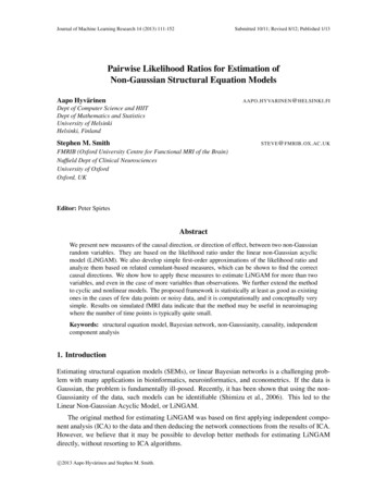
H YV ÄRINEN AND S MITHThe regression coefficient ρ is always smaller than one in absolute value, and thus ρ2 ρ4 0.Assuming that the relevant kurtosis is positive, which is very often the case for real data, the signof R̃c4 can be used to determine the causal direction in the same way as in the case of the likelihoodapproximation R̃ in (5). Thus, the cumulant-based approach allowed us to prove rigorously that anonlinear correlation of the form (6) can be used to infer the causal direction, since it takes oppositesigns under the two models. Note that this nonlinear correlation has exactly the same algebraicform as the likelihood ratio approximation (5); only the nonlinear scalar function is different. Inparticular, this analysis shows that the exact form of the nonlinearity is not important: the cubicnonlinearity is valid for all distributions of positive kurtosis.If the relevant kurtosis is negative, a simple change of sign is needed. In general, we should thusmultiply R̃c4 by the sign of the kurtosis to obtainR̃′c4 (x, y) sign(kurt(x))ρÊ{x3 y xy3 }.Here, we get the complication that we have to choose whether we use the sign of the kurtosis of xor y. Usually, however, the signs would be the same, and we might have prior information on theirsign, which is in most applications positive.2Related cumulant-based measure were proposed by Dodge and Rousson (2001) and Dodge andYadegari (2010). Their fourth-order measures used the ratio of marginal kurtoses, as opposed tothe cross-cumulants we use here. They further assumed the disturbances to be Gaussian (or at leastto have zero cumulants), which makes their measures less general than ours. In fact, their methodrelies on the fact that kurtosis is decreased by adding a Gaussian disturbance, but if the disturbanceis much more kurtotic than the regressor, the opposite can be the case.2.7 Intuitive InterpretationsNext, we provide some intuitive interpretations of the obtained first-order approximations of thelikelihood ratio.2.7.1 G RAPHICAL I NTERPRETATIONThe cumulants and nonlinear correlations have a simple intuitive intepretation. Let us consider thecumulant first. The expectations E{x3 y} or E{xy3 } are basically measuring points where both xand y have large values, but in contrast to ordinary correlation, they are strongly emphasizing largevalues of the variable which is raised to the third power.Assume the data follows x y, and that both variables are sparse (super-Gaussian). Then, bothvariables simultaneously have large values mainly in the cases where x takes a large value, makingy large as well. Now, due to regression towards the mean, that is, ρ 1, the value of x is typicallylarger than the value of y. Thus, E{x3 y} E{xy3 }. This is why E{x3 y} E{xy3 } 0 under x y.The idea is illustrated in Figure 1.2. In the general case where the (real) kurtoses of x and y are allowed to have different signs, we need to computetwo quantities: R̃′c4 (x, y) sign(kurt(x))ρÊ{x3 y xy3 } and R̃′c4 (y, x) sign(kurt(y))ρÊ{y3 x yx3 }. According tothe analysis above, the former quantity is positive if x y, and the latter quantity is positive if y x. However, inpractice, this does not lead to a simple decision rule since due to finite sample size, or violations of the model, itcould be that both of these quantities are positive, or none of them. In such cases, the decision rule should be definedso as to indicate that the causal direction could not be decided.118
PAIRWISE L IKELIHOOD R ATIOS FOR N ON -G AUSSIAN SEM SyxFigure 1: Intuitive illustration of the nonlinear correlations. Here, x y and the variables are verysparse. The nonlinear correlation E{x3 y} is larger than E{xy3 } because when both variables are simultaneously large (the “arm” of the distribution on the right and the left), xattains larger values than y due to regression towards the mean.This interpretation is valid for the tanh-based nonlinear correlation as well, because we can usethe function h(u) u tanh(u) instead of tanh to measure the same correlations but with oppositesign. In fact, we haveR̃sparse ρÊ{h(x)y x h(y)}because the linear terms cancel each other. The function h is a soft thresholding function, and thushas the same effect of emphasizing large values as the third power. Thus the same logic applies forh and the third power.2.7.2 I NTERPRETATIONAS I MPLICATIONEven if the data is not assumed to follow any particular model, the nonlinear correlation could beinterpreted as a logical implication. In general, if the existence of event A implies the existence ofevent B, but there is no implication in the other direction, a causal influence from A to B might beinferred. Since A B is equivalent to B A, there has to be some clear distinction between theevents and their negations for this interpretation to be meaningful. We assume here that the eventsare rare, that is, have small probabilities.Now, let us consider the events A, defined as “x takes a very large value” and B, defined as “ytakes a relatively large value of the same sign as x”. Notice that because the regression coefficientis smaller than one, we cannot require y to take particularly large values. It is assumed here that thethresholds for deciding when a value is large are chosen so that both of these events are rare.To investigate implication, we can consider how to refute it. To refute A B, we should considercases where x takes a very large value but y takes a value of the opposite sign. This can be measuredby Ex3 ( y) where x3 looks at large values of x and the minus sign changes this into a measure ofhow much large values of x coexist with y’s of opposite sign.119
H YV ÄRINEN AND S MITHThus, Ex3 y Exy3 can be seen as measuring of how much evidence we have to refute y x(latter term) minus the evidence to refute x y (negative of first term). If it is large, we accept theimplication x y together with its causal interpretation.It might be argued that the connection between causality and implication could also plausiblybe defined in the opposite direction: If A implies B as defined above, then B causes A. However,we shall now argue that the interpretation we gave above follows naturally from the definition of aSEM with two variables. Assume x y and ρ 0. If x is very large, y is likely to be large and ofthe same sign, since it is not very probable that d would cancel out the effect of ax. Thus, we haveA B when x causes y under the SEM framework.2.8 Noise-Tolerance of the Nonlinear CorrelationsAn interesting point to note is that the cumulant in (6) is, in principle, immune to additive measurement noise. Assume that instead of the real x, y, we observe noisy versions x̃ x n1 and ỹ y n2where the noise variables are independent of each other and x and y. By the basic properties ofcumulants (see proof of Theorem 1), the nonlinear correlations are not affected by the noise at all inthe limit of infinite sample size. Thus, our method in not biased by noise. This is in stark contrast toICA algorithms which are strongly affected by additive noise; thus ICA-based LiNGAM (Shimizuet al., 2006) would not yield consistent estimators in the presence of noise.To be more precise, we haveE{x̃3 ỹ} E{x̃ỹ3 } cum(x̃, x̃, x̃, ỹ) cum(x̃, ỹ, ỹ, ỹ) cum(x, x, x, y) cum(x, y, y, y) E{x3 y} E{xy3 }due to the independence of n1 and n2 of the other variables and each other.On the other hand, the estimation of ρ is strongly affected by the noise. This implies that R̃c4 isnot immune to noise. Nevertheless, measurement noise would only decrease the absolute value ofρ and not change its sign. Thus, the sign of R̃c4 is not affected by additive measurement noise in thelimit of infinite sample. This applies for both Gaussian and non-Gaussian noise.The fact that the ρ is only a multiplicative scaling in the nonlinear correlations (6) or (5) mustbe contrasted with its role in the likelihood ratio (1) where its effect is more complicated. Thus,when ρ is underestimated due to measurement noise, it may have a stronger effect on the likelihoodratio, while its effect on the nonlinear correlations is likely to be weaker. While this logic is quiteapproximative, simulations below seem to support it.On the other hand, the standardization of the variables is also affected by noise, in particular ifthe noise variances are not equal. As long as the noise variances are equal, the error in standardization will affect the measures by a multiplicative constant only, effectively making the cumulantssmaller. Thus, the noise-tolerance of the cumulants may be useful in practice only if the variancesof the noise variables are equal.2.9 Skewed VariablesAbove, the likelihood ratio approximations and cumulants were developed for sparse, typicallysymmetrically-distributed variables. Here, we consider the extension to skewed variables. Again,the underlying motivations is that if we know the distributions are skewed, we can use this priorknowledge to obtain particularly simple measures of causal direction. The cumulant-based analysis120
PAIRWISE L IKELIHOOD R ATIOS FOR N ON -G AUSSIAN SEM Sis mainly for theoretical interest due to the sensitivity of cumulants to outliers; we provide a morerobust nonlinearity for analysing real data.2.9.1 C UMULANT-BASED A PPROACHThe cumulant-based approach allows for a very simple extension of the framework to skewed variables. As a simple analogue to (6), we can define a third-order cumulant-based statistic as followsR̃c3 (x, y) ρÊ{x2 y xy2 }.(10)The justification for this definition is in the following theorem, which is the analogue of Theorem 1:Theorem 2 If the causal direction is x y, we haveR̃c3 skew(x)(ρ2 ρ3 )(11)and if the causal direction is the opposite, we haveR̃c3 skew(y)(ρ3 ρ2 ).(12)Proof Consider the third-order cumulantC(x, y) cum(x, x, y) Ex2 ywhere we assume the two variables are standardized. We have skew(x) C(x, x) cum(x, x, x).The nonlinear correlation can be expressed using this cumulant asR̃c3 ρ[C(x, y) C(y, x)].Assuming the causal direction is x y, we haveR̃c3 ρ[cum(x, x, ρx d) cum(x, ρx d, ρx d)] ρ[ρ cum(x, x, x) cum(x, x, d) ρ2 cum(x, x, x) 2ρ cum(x, x, d) cum(x, d, d)] ρ[ρ skew(x) ρ2 skew(x)] skew(x)[ρ2 ρ3 ]which proves (11). The proof of (12) is again completely symmetric.To use the measure (10) in practice, we have to take into account the fact that we cannot assume,in general, the skewnesses of the variables to have some particular sign. In some applications this ispossible: For example, in resting-state fMRI data it might be safe to assume that the skewnesses areall positive because it is much more common that the signals obtain large values due to activationthan due to inhibition (however, this point needs to be confirmed by empirical investigations offMRI data).In the general case, we propose that before computing these nonlinear correlations, the signsof the variables are first chosen so that the skewnesses are all positive. This can be accomplishedsimply by multiplying the variables by the signs of their skewnesses to get a new variable x x sign(skew(x)) x121(13)
H YV ÄRINEN AND S MITHand the same for y (this t
model (LiNGAM). We also develop simple first-order approximations of the likelihood ratio and analyze them based on related cumulant-based measures, which can be shown to find the correct causal directions. We show how to apply these measures to estimate LiNGAM for more than two variables, and even in the case of more variables than observations.