Transcription
tt --Massachusetts Institute of TechnologyMIT Video COurseVideo Course Study GuideFinite ElementProcedures for Solidsand Structures Linear AnalysisKlaus-JOrgen BatheProfessor of Mechanical Engineering, MITPublished by MIT Center for Advanced Engineering studyReorder No 672-2100
PREFACEThe analysis of complex static and dynamic problems in volves in essence three stages: selection of a mathematicalmodel, analysis of the model, and interpretation of the results.During recent years the finite element method implemented onthe digital computer has been used successfully in modelingvery complex problems in various areas of engineering andhas significantly increased the possibilities for safe and cost effective design. However, the efficient use of the method isonly possible if the basic assumptions of the proceduresemployed are known, and the method can be exercisedconfidently on the computer.The objective in this course is to summarize modern andeffective finite element procedures for the linear analyses ofstatic and dynamic problems. The material discussed in thelectures includes the basic finite element formulations em ployed, the effective implementation of these formulations incomputer programs, and recommendations on the actual useof the methods in engineering practice. The course is intendedfor practicing engineers and scientists who want to solve prob lems using modem and efficient finite element methods.Finite element procedures for the nonlinear analysis ofstructures are presented in the follow-up course, Finite ElementProcedures for Solids and Structures - Nonlinear Analysis.In this study guide short descriptions of the lectures andthe viewgraphs used in the lecture presentations are given.Below the short description of each lecture, reference is madeto the accompanying textbook for the course: Finite ElementProcedures in Engineering Analysis, by K.J. Bathe, Prentice Hall, Inc., 1982.The textbook sections and examples, listed below theshort description of each lecture, provide important readingand study material to the course.
ContentsLecturesl.Some basic concepts of engineering analysis1-12.Analysis of continuous systems; differential andvariational formulations2-13.Formulation of the displacement-based finite element method3-14.Generalized coordinate finite element models4-15.Implementation of methods in computer programs;examples SAp, ADINA5-16.Formulation and calculation of isoparametric models6-17.Formulation of structural elements7-18.Numerical integrations, modeling considerations8-19.Solution of finite element equilibriumequations in static analysis9-1Solution of finite element equilibriumequations in dynamic analysis10-11l.Mode superposition analysis; time history11-112.Solution methods for calculations offrequencies and mode shapes12-110.
SOME BASICCONCEPTS OFENGINEERINGANALYSISLECTURE 146 MINUTESI-I
SolIe basic ccnacepls of eugiDeeriDg ualysisLECTURE 1 Introduction to the course. objective of lecturesSome basic concepts of engineering analysis.discrete and continuous systems. problemtypes: steady-state. propagation and eigen value problemsAnalysis of discrete systems: example analysis ofa spring systemBasic solution requirementsUse and explanation of the modern direct stiff ness methodVariational formulationTEXTBOOK: Sections: 3.1 and 3.2.1. 3.2.2. 3.2.3. 3.2.4Examples: 3.1. 3.2. 3.3. 3.4. 3.5. 3.6. 3.7. 3.8. 3.9.3.10. 3.11. 3.12. 3.13. 3.141-2
Some basic concepts 01 engineering aulysisINTRODUCTION TO LINEARANALYSIS OF SOLIDS AND STRUCTURES The finite element method is nowwidely used for analysis of structuralengineering problems. 'n civil, aeronautical, mechanical,ocean, mining, nuclear, biomechani cal,. engineering Since the first applications twodecades ago,- we now see applicationsin linear, nonlinear, staticand dynamic analysis.- various computer programsare available and in significantuseMy objective in this set oflectures is: to introduce to you finiteelement methods for thelinear analysis of solidsand structures.["Iinear" meaning infinitesi mally small displacements andlinear elastic material proeer ties (Hooke's law applies)j to consider- the calculation of finiteelement matrices- methods for solution of thegoverning equations- computer implementations.to discuss modern and effectivetechniques, and their practicalusage.- the formulation of the finiteelement equilibrium equations1·3
Some basic concepts of engineering analysisREMARKS Emphasis is given to physicalexplanations rather than mathe matical derivations Techniques discussed are thoseemployed in the computer pro gramsSAP and ADINASAP Structural Analysis ProgramADINA Automatic DynamicIncremental Nonlinear Analysis These few lectures represent a verybrief and compact introduction tothe field of finite element analysis We shall follow quite closelycertain sections in the bookFinite Element Proceduresin Engineering Analysis,Prentice-Hall, Inc.(by K.J. Bathe).Finite Element Solution ProcessPhysical problem. - - Establish finite elementmodel of physicalproblemRevise (refine)the model?I:I,- S ol v e th e m o d elI -1-41- - iL- I n te r.;.p re t t h e re s u lt S .J
SolIe basic concepts of engiDeering analysis10 ft15 ftI,.12 at 15 Analysis of cooling tower.K - ,-Fault\\(no restraint assumed)Altered' gritE toEc.,Analysis of dam.1·5
Some basic concepts of engineering analysisB.t Wo.E ;;C -------FFinite element mesh for tireinflation analysis.1·6
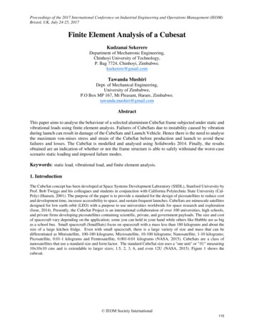
SolDe basic concepts of engineering analysisSegment of a spherical cover of alaser vacuum target chamber.pl,Wp-0.2PINCHED CYLINDRICALSHELLOD;:.,.----.--- C 16x 16 MESHMilEtW -50P- 100"" 0.1-150 CBENDING MOMENT DISTRIBUTION ALONG DC OFPINCHED CYLINDRICAL SHELL 16x 16 MESH-200 DISPLACEMENT DISTRIBUTION ALONG DC OFPINCHED CYLINDRICAL SHELL1-7
SoBle basic concepts 01 engineering analysisIFinite element idealization of windtunnel for dynamic analysisSOME BASIC CONCEPTSOF ENGINEERINGANALYSISThe analysis of an engineeringsystem requires:- idealization of system- formulation of equili brium equations- solution of equations- interpretation of results1·8
Some basic concepts of engineering analysisSYSTEMSDISCRETECONTINUOUSresponse isdescribed byvariables at afinite numberof pointsresponse isdescribed byvariables atan infinitenumber ofpointsset of alge braic - equationsset of differ entialequationsAnalysis of complex continu ous system requires solution ofdifferential equations usingnumerical proceduresPROBLEM TYPES ARE STEADY -STATE (statics) PROPAGATION (dynamics) EIGENVALUEFor discrete and continuoussystemsANALYSIS OF DISCRETESYSTEMSSteps involved:reduction of continuoussystem to discrete form- system idealizationinto elementspowerful mechanism:- evaluation of elementequilibrium requirementsthe finite element methods,implemented on digitalcomputers- element assemblage- solution of response1·9
Some basic concepts of engineering analysisExample:steady - state analysis ofsystem of rigid cartsinterconnected by springsPhysical layoutELEMENTSU3U1I : \l)1,F(4)1k, u1 -- F(' )u2-,'2 [34' ].[F1'4 [-11-1]["1]1 UF(4)31-1]["I]fF}]1 uF( 2 )-12u,2u2k33'3 [ ]-1-r ]f1F(S)2F(S)331PuF(3)l]2-2[F(5l]'5 [-11-t]1 u F1S )F(3)-- 2F(3)1·10F(4)F(2 )--- 2F(2)---,.23
SolIe basic cOIcepls of engineering analysisElement interconnectionrequirements :F(4) F(S) R333These equations can bewritten in the formKU E.Equilibrium equationsKU R(a)TU [u1T [R-R1K·· k4···k k k -k - k. 1 2 3.·'" .2.3 .: .-k.4 . .··. -k 2 - k3 k2 k3 k S -k S·. . . . .··.1·11
Some basic concepts of engineering analysisand we note that ti 1 (i)where: :]o0etc .This assemblage process iscalled the direct stiffnessmethodThe steady- state analysis iscompleted by solving theequations in (a)1·12
Some basic concepls 01 engineering analysisu,·. :·:. .········. u,.K1K .::. .····.:·.U1. : . K . :. 1---.JI.l\fl--r/A ,1\1\1\ r/A1·13
SOlDe basic concepts of engineering analysisu,·:····.K .:.'O ··u, K4 ;K 1 K 2 K 3 ;-K 2 -K O'O'O'O'OK 'O'O . u,K4 ;K 1 K 2 K 3 -K2 -K 3-K4'O'O K -K 2 -K 3 K2 K3 K5'O'O :I1·14K-K5
Some basic concepts of engineering analysisIn this example we usedthe direct approach; alternativelywe could have used a variationalapproach.In the variational approach weoperate on an extremumformu lation:u W strain energy of systemtotal potential of theloadsEquilibrium equations are obtainedfroman - -0(b)1In the above analysis we haveU UT!!!TW U RInvoking (b) we obtainKU RNote: to obtain U and W weagain add the contributions fromall elements1·15
SOlDe basic concepts of engineering analysisPROPAGATION PROBLEMSmain characteristic: the responsechanges with time need toinclude the d'Alembert forces:For the example:m,aaM a am2 aa m3EIGENVALUE PROBLEMSwe are concerned with thegeneral ized eigenvalue problem(EVP)Av ABv!l , .!l are symmetric matricesof order nv is a vector of order nA is a scalarEVPs arise in dynamic andbuckling analysis1·16
Some basic concepts of engineering analysisExample: system of rigid carts lU KU OLetU p sin W(t-T)Then we obtainw2 sin W(t-T) -K p-sin W(t-T) -0Hence we obtain the equationThere are 3 solutionsw,, ,(l)2 ' 2eigenpairsw3 ' 3In general we have n solutions1·17
ANALYSIS OFCONTINUOUS SYSTEMS;DIFFEBENTIAL ANDVABIATIONALFOBMULATIONSLECTURE 259 MINUTES2-1
Analysis 01 continnous systems; differential and variational lonnDlationsLECTURE 2Basic concepts in the analysis of continuoussystemsDifferential and variational formulationsEssential and natural boundary conditionsDefinition of em-I variational problemPrinciple of virtual displacementsRelation between stationarity of total potential, theprinciple of virtual displacements, and the differ ential formulationWeighted residual methods, Galerkin, leastsquares methodsRitz analysis methodProperties of the weighted residual and RitzmethodsExample analysis of a nonuniform bar, solutionaccuracy, introduction to the finite elementmethodTEXTBOOK:Sections: 3.3.1, 3.3.2, 3.3.3Examples: 3.15, 3.16, 3.17, 3.18, 3.19, 3.20, 3.21,3.22, 3.23, 3.24, 3.252·2
Analysis of continuous systems; differential and variational formulationsBASIC CONCEPTSOF FINITEELEMENT ANALYSIS CONTINUOUS SYSTEMS Some additionalbasic concepts areused in analysis ofcontinuous systems We discussed somebasic concepts ofanalysis of discretesystemsCONTINUOUS ontRitz MethodWeighted residualmethodsGalerkin . -----41 least squares.finite element method2·3
Analysis of continuous systeDlS; differential and ,arialionalIOl'llulali.Example - Differential formulation/ Lt: )Young's modulus, Emass density,cross-sectional area, AR. -------The problem governing differentialequation isDerivation of differential equationThe element force equilibrium require ment of a typical differential elementis using d'Alembert's principler .-; dxI Area A, mass densityIaA Ix A adx - aA IxoX Xp pThe constitutive relation isaau E axCombining the two equations abovewe obtain2·4A2au
baIysis 01 COitiDlOU systems; differatial aDd variationaliOl'lDDlatiODSThe boundary conditions areu(O,t} EA (L,t) RO9 essential (displ.) B.C.9 natural (force) B.C.with initial conditionsu(x,O} at (x ' O) In general, we havehighest order of (spatial) deriva tives in problem-governing dif ferential equation is 2m.highest order of (spatial) deriva tives in essential b.c. is (m-1)highest order of spatial deriva tives in natural b.c. is (2m-1)Definition:We call this problem a Cm-1variational problem.2·5
Analysis 01 continuous systems; differential and variatioD,a1 fOl'llolatiODSExample - Variational formulationWe have in generalII U-WFor the rodfLII J } EAoau 2(--)axdx -iLu fBdx - uoando 0uand we have 0 II 0The stationary condition 6II 0 givesrLauaurL.BJO(EA ax)(6 ax) dx -)0 6u t- dx- 6uLR 0This is the principle of virtualdisplacements governing theproblem. In general, we writethis principle asor(see also Lecture 3)2·6LR
lIiIysis of .IiDIGUS systems; differential and variatiooallormulatioDSHowever, we can now derive thedifferential equation of equilibriumand the b.c. at x l .Writinga8uax8 aufor, re-axcalling that EA is constant andusing integration by parts yieldsdx [EA- EA \dX Iax x Lx oSince QUO is zero but QUisarbitrary at all other points, wemust haveandau I x L REAaxAlso,fBa2u -A p -at 2andhence we have2·7
Analysis of cODtiDaoas syst diIIereatial and variatioul fOlllalatiODSThe important point is that invokingo IT 0 and using the essentialb.c. only we generate the principle of virtualdisplacements the problem-governing differ ential aquatio!) the natural b.c. (these are inessence "contained in" IT ,i.e., inW).In the derivation of the problem governing differential equation weused integration by parts the highest spatial derivativein IT is of order m . We use integration by partsm-times.Total Potential ITIUse oIT 0 and essential "b.c. Principle of VirtualDisplacementssolveproblemIIntegration by parts Differential Equationof Equilibriumand natural b.c.2·8solveproblem
balysis of aDa. syst-: diBerential and variatiouallnaiatiOlSWeighted Residual MethodsConsider the steady-state problem(3.6)with the B.C.B.[ / ] 1q.,1 1 ,2, at boundary (3.7)iThe basic step in the weightedresidual (and the Ritz analysis)is to assume a solution of theform(3.10)where the f i are linearly indepen dent trial functions and the aiare multipliers that are deter mined in the analysis.Using the weighted residual methods,we choose the functions f i in (3.10)so as to satisfy all boundary conditionsin (3.7) and we then calculate theresidual,nR r - L2mCL a· f.]1 111(3.11 )The various weighted residual methodsdiffer in the criterion that they employto calculate the ai such that R is small.In all techniques we determine the aiso as to make a weighted average ofR vanish.2·9
Analysis 01 C.tinnoDS systems; differential and variational 10000nlationsGalerkin methodIn this technique the parameters ai aredeterm ined from the n equationsfD f.R dD O; 1,2, ,n(3.12)1Least squares methodIn this technique the integral of thesquare of the residual is minimized withrespect to the parameters ai 'aaa.1; 1,2, ,n[The methods can be extended tooperate also on the natural boundaryconditions, if these are not satisfiedby the trial functions.]RITZ ANALYSIS METHODLet n be the functional of theem-1 variational problem that isequivalent to the differentialformulation given in (3.6) and (3.7).In the Ritz method we substitute thetrial functions p given in (3.10)into n and generate n simul taneous equations for the para meters ai using the stationarycondition on n ,anaa.12·10 0; 1,2, ,n(3.14)
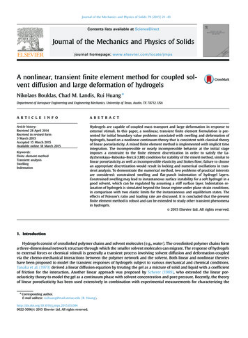
Analysis of continuous systems; differential and variational formulationsProperties The trial functions used in theRitz analysis need only satisfy theessential b.c. Since the application of oIl 0generates the principle of virtualdisplacements, we in effect usethis principle in the Ritz analysis. By invoking 0 II 0 we minimizethe violation of the internal equilibriumrequirements and the violation ofthe natural b.c. A symmetric coefficient matrixis generated, of formKU RExampleArea 1 em2(. x,u.F---- --.;;B;",.,.---- -R 100 N ---r;;;- -e-CI-.-- ---·-I.- -------·-I100 em80 emFig. 3.19. Bar subjected toconcentrated end force.2·11
Analysis of COitiDlOIS systems; differeatial ad ,ariali" fOllDaialiODSHere we have180112 EA( )2ax ITodx -100 u Ix 180and the essential boundary conditionis u Ix O 0Let us assume the displacementsCase 1 a1xu a2iCase 2 I1JOu0 x 100100 x 180We note that invokingwe obtain180(EA1oIT oIT 0 ) o( )odx - 100 OU Ix 180 0or the principle of virtualdisplacements180 oJET-V2·12( u)( EA )T-dV IT. F.11Idx 100 OU x 180
Analysis of continuous systems; differential and variational formulationsExact SolutionUsing integration by parts weobtain ax(EAEA ax )ax 0 100x 180The solution isu 1 O x ; 0 x 100100 x 180The stresses in the bar area 100;a 0 x 100100; 100 x 180(l x-l00)2402·13
Analysis of continuous systems; differential and variational formulationsPerforming now the Ritz analysis:Case 1dx I2f180100I nvoking thatorr 0E [0.4467116we obtain34076116anda1 128.6--- E ---a 2 -- - 0.341EHence, we have the approximatesolution2·14u a 12C.6Ex -0.341E128.6 - 0.682 x2x(1 x-l00)240
Analysis of continuous systems; differential and variational formulationsCase 2Here we haveJ100En 2aEf(1 x -l00)240100Invoking again24018012(100 u B) dx I2on 0[15.4 -13]-13we obtain[ :] [ oo] 13Hence, we now haveUB 10000EUc11846.2Eando 1000 x 100o 1846.2 23.0880x 1002-15
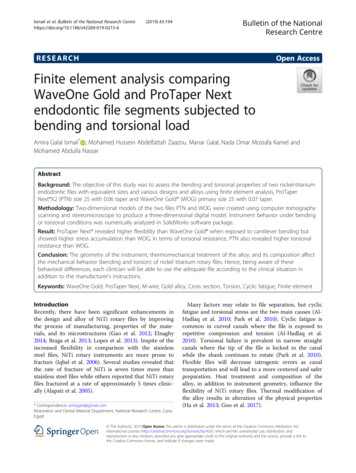
Aulysis of COilinDmas systems; diUerenliai and varialiOlla1I01'1BDlaIiGlSuEXACT15000-- --- E-::.:-- 10000 .-.-.E"Sol ution 25000-E.,- --r- --.,r------.I X180100CALCULATED DISPLACEMENTS(J100 -I ::: - : os: , ""50"I I- ,JL. . .- EXACTSOLUTION 1 . .---, --------r------- X100CALCULATED STRESSES2·18SOLUTION 2180
balysis of coatiDloas systms; diBerenlial ud variational fonnllatioasWe note that in this last analysise we used trial functions that donot satisfy the natural b.c.e the trial functions themselvesare continuous, but the deriva tives are discontinuous at pointB.1for a em- variational problemwe only need continuity in the(m-1)st derivatives of the func tions; in this problem m 1 .edomains A - Band B - e arefinite elements andWE PERFORMED AFINITE ELEMENTANALYSIS.2·17
FORMULATION OF THEDISPLACEMENT-BASEDFINITE ELEMENTMETHODLECTURE 358 MINUTES3·1
Formulation of the displacement-based finite element methodLECTURE 3 General effective formulation of the displace ment-based finite element methodPrinciple of virtual displacementsDiscussion of various interpolation and elementmatricesPhysical explanation of derivations and equa tionsDirect stiffness methodStatic and dynamic conditionsImposition of boundary conditionsExample analysis of a nonuniform bar. detaileddiscussion of element matricesTEXTBOOK: Sections: 4.1. 4.2.1. 4.2.2Examples: 4.1. 4.2. 4.3. 4.43·2
Formulation of the displacement-based finite element methodFORMULATION OFTHE DISPLACEMENT BASED FINITEELEMENT METHOD- A very generalformu lation-Provides the basis ofalmost all finite ele ment analyses per formed in practice-The formulation isreally a modern appli cation of the Ritz/Gelerkin proceduresdiscussed in lecture 2-Consider static anddynamic conditions, butlinear analysisFig. 4.2. General three-dimensional body.3·3
FOl'Dlulation of the displaceDlent·based finite e1mnent lDethodThe external forces arefBXfB fByfSfBf iFX fSyFi FyifSiFZZZ(4.1)The displacements of the body fromthe unloaded configuration aredenoted by U, whereuT [uVw](4.2)The strains corresponding to U are, T [E XX Eyy EZZ YXy YyZ YZX]and the stresses corresponding toare3·4 (4.3)
Formulation of the displacement-based finite element methodPrinciple of virtual displacementswhereITT [IT If w](4.6 )Fig. 4.2. General three-dimensional body.3·5
Formulation of the displaceaenl-based filile e1eDlenl .ethod,,x,u""Finite elementFor element (m) we use:!!(m) (x, y, z)"T!! [U, V, W,z)0(4.8)U2V2W2 UNVNW N]!!"T [U,U 2U3. Un]§.(m) (x, y, z) (m) (x, y,!.(m)3·& !:!.(m) (x, y, f(m) (m) -rI(m)(4.9)z)!!(4.'0)(4.'1)
'OI'IIalation of the displaceDlenl-based filile eleDlenl methodRewrite (4.5) as a sum of integrationsover the elements(4.12)Substitute into (4.12) for the elementdisplacements, strains, and stresses,using (4.8), to (4.10),---.ll.c -----Ij-'iTlIf 1B(m) Tc(m)B(m)dv(m)j U v(m) l-j [ITI 1"-(m) T-- 1L l(m)T (m)!!(m) 1.BdV(m)j---- (m) f.(m) (m)-mVI, .( )TB(m)TTI(m) dv(m)jm- .r .1" I:::-- m:,. L f. ) !!sCm)Ti m)dScmljmm JV.:. , IEl;rm) - B(m) l.u·)(- )(m)y:(m) !!(m) (m) T-US-(m) T------. (4.13)3·7
Formulation of the displacement-based finite element .ethodWe obtainKU R(4.14)whereR .Ba Rs - R1 fK J-( 4. 15)B(m)Tc(m)B(m)dV(m)(4.16)m V(m)- -R "'1. lm) -H(m)TfB(m)dV(m)(4.17)-"'1 "'1-1R -SRR HS (m)Tfs(m)dS(m) (4.18) m) B(m)TT1(m)dV(m) V(m) -(4.19) -F(4.20)In dynam ic analysis we have B f(m)T -B(m)V(m) .!:!.[1.p(m).!:!.(m) ]dV(m)MD KU R3·8B(m)1.(4.21 )(4.22)-B(m) 1. (m)- p!!
Formulation of the displacement-based finite element methodTo impose the boundary conditions,we use a b a b at!t b- (4.38). a a - b - b (4.39) a b a b (4.40)i!I! AV-Global degreesof freedom; VI (restrained\LCOST ['/.TransformedC,-: :e)rl'fua -sina]sin aU T\eedomdegrees offcos aITFig. 4.10. Transformation to skewboundary conditions3·9
Formulation of the displacement-based finite element method.th1columnFor the transformation on thetotal degrees of freedom we use1. i th row(4.41 )so thatj1cos a.T .Mu Ku R(4.42)}hsin a.whereLFig. 4.11. Skew boundary conditionimposed using spring element.We can now also use this procedure(penalty method)Say Ui b, then the constraintequation is,k U. k bwherek » k ."3·10(4.44).thJ!-s ina.1cos a.1
FormDlation of the displacement·based finite element methodExample analysisareaz 1100xyarea 910080element Finite elementsJ I"-I10080 I3·11
Formulation of the displacement·based finite element methodElementinterpolation functions1.0I .--ILDisplacement and straininterpolation matrices:H(l} [(l-L)-100!:!.(2} [a!!(l) [!!(2) [3·12y100(1- L)a]v(m} H(m}U80:0]11001100a]a180180]av B(m}Uay -
FOI'IDDlation of the displacement·based finite element methodstiffness matrix- 11005. (1 HEllOal O [-l O l Oo}YaU1- 80180HenceE 240[ 2.4-2.4-2.415.4a-13Similarly for M '.!!B ' and so on.Boundary conditions must still beimposed.3·13
GENERALIZEDCOORDINATE FINITEELEMENT MODELSLECTURE 457 MINUTES4·1
Generalized coordinate finite element modelsLECTURE 4 Classification of problems: truss, plane stress, planestrain, axisymmetric, beam, plate and shell con ditions: corresponding displacement, strain, andstress variablesDerivation of generalized coordinate modelsOne-, two-, three- dimensional elements, plateand shell elementsExample analysis of a cantilever plate, detailedderivation of element matricesLumped and consistent loadingExample resultsSummary of the finite element solution processSolu tion errorsConvergence requirements, physical explana tions, the patch testTEXTBOOK: Sections: 4.2.3, 4.2.4, 4.2.5, 4.2.6Examples: 4.5, 4.6, 4.7, 4.8, 4.11, 4.12, 4.13, 4.14,4.15, 4.16, 4.17, 4.184-2
Generalized coordinate finite eleDlent modelsDERIVATION OF SPECIFICFINITE ELEMENTS Generalized coordinatefinite element models (m) iIn essence, we needB(m)T C(m) B(m) dV (m)aW) JH(m) B (m) C (m)-V(m),-'-H(m)T LB(m) dV (m)V(m)R(m)!!S fSHS(m)T f S(m) dS (m)- Convergence ofanalysis results(m) -etc.AAcross section A-A:TXX is uniform.All other stress componentsare zero.Fig. 4.14. Various stress and strainconditions with illustrative examples.(a) Uniaxial stress condition: frameunder concentrated loads.4·3
Ge.raJized coordiDale finite elementlDOIIeIsHale\I\-61ZII\-\\' Tyy , TXY are uniformacross the thickness.All other stress componentsare zero.TXXFig. 4.14. (b) Plane stress conditions:membrane and beam under in-planeactions.u(x,y), v(x,y)are non-zerow 0 , E zz 0Fig. 4.14. (e) Plane strain condition:long dam subjected to water pressure.4·4
Generalized coordinate finite element modelsStructure and loadingare axisymmetric.j(IIII,I\-IAll other stress componentsare non-zero.Fig. 4.14. (d) Axisymmetric condition:cylinder under internal pressure./(before deformation)(after deformation)SHELLFig. 4.14. (e) Plate and shell structures.4·5
Generalized coordinate finite element modelsDisplacementComponentsProblemuwBarBeamPlane stressPlane strainAxisymmetricThree-dimensionalPlate Bendingu, vu, vu,vu,v, wwTable 4.2 (a) Corresponding Kine matic and Static Variables in VariousProblems.-Strain Vector TProblem(E".,)Bar[IC.,]BeamPlane stress(E"., El'l' )' "7)Plane strain(E., EJ"7 )'.7)Axisymmetric[E., E"77 )'''7 Eu )Three-dimensional [E., E"77 Eu )'''7 )'76Plate Bending(IC., 1(77 1("7).)'.,)auau aua/ )'''7 ayax'awawaoyw , IC., -dx ' IC - OyZ,IC., 2Nolallon:E.au ax' 7 11Z7710xTable 4.2 (b) Corresponding Kine matic and Static Variables in VariousProblems.4·&
Generalized coordinate finite element modelsProblemStress Vector 1:TBarBeamPlane stressPlane strainAxisymmetricThree-dimensionalPlate Bending[T;u,][Mn ][Tn TJIJI T"'JI][Tn TJIJI T"'JI][Tn TJIJI T"'JI Tn][Tn TYJI Tn T"'JI TJI' Tu ][MnMJIJI M"'JI]Table 4.2 (e) Corresponding Kine matic and Static Variables in VariousProblems.ProblemMaterial Matrix. BarBeamPlane StressE1-1':&EEl1 vv 1[o 0 1 .]Table 4.3 Generalized Stress-StrainMatrices for Isotropic Materialsand the Problems in Table 4.2.4·7
Generalized coordinate finite element modelsELEMENT DISPLACEMENT EXPANSIONS:For one-dimensional bar elementsFor two-dimensional elements(4.47)For plate bending elementsw(x,y) Y,2 Y2 x Y3Y Y4xy Y5x .(4.48)For three-dimensional solid elementsu (x,y,z) a, Ozx Y Ci4Z xy .w(x,y,z) Y, y 2x y y y z y xy .345(4.49)4·8
Generalized coordinate finite element modelsHence, in generalu (4.50)ex(4.51/52)(4.53/54)(4.55)ExamplerlpNodal point 69Element005Y.VY.Vla) Cantilever plate@CDV7741X.V8V7X.V(bl Finite element idealizationFig. 4.5. Finite element planestress analysis; i.e. T T TZZZyZX 04·9
Generalized coordinate finite element modelsLJ2. US2--II--.- - - - - - - - -. Element nodal point no. 4nodal pointno. 5 . structureelement Fig. 4.6. Typical two-dimensionalfour-node element defined in localcoordinate system.For element 2 we haveU{X,y)] (2)[ v{x,y)whereuT [U 1-4·10 H(2) u--
Generalized coordinate linite element modelsTo establish H (2) we use:orU(X,y)][ v(x,y) l!.where [ ! }! [1x y xy]andDefiningwe haveQ Aa.HenceH iPA- 14·11
Generalized coordinate finite element modelsHenceH- fll4(1 x ) ( Hy) ::aI Ia:I: (1 x )( 1 y) :andzt':U3 U4 UsU6UJH'ZJ- [00U2I0 : H IJVJU: H ZI(a)U7 Us:HI.H 16HIs: 0H zs : 0Element layout00:Hu :Ha :UIS -assemblage degreeszeroszeros(b)OJ offreedomO2x18Local-global degrees of freedomFig. 4.7. Pressure loading onelement (m)4·12v.U9 U1a0 0: HI.o : H ZJ H 21 : H:: H: 6 : 0 0: H.VI -element degrees of freedomH 17Ull U12 U1 3 U14:H IIu.
Generalized coordinate finite element modelsIn plane-stress conditions theelement strains arewhereE- au . E av.au avxx - ax' yy - ay , Yxy - ay axHencewhereI [ I1 0 y'OI000 1I 001XI10I4·13
Generalized coordinate finite element modelsACTUAL PHYSICAL PROBLEMGEOMETRIC DOMAINMATERIALLOADINGBOUNDARY CONDITIONS1MECHANICAL IDEALIZATIONKINEMATICS, e.g. trussplane stressthree-dimensionalKirchhoff plateetc.MATERIAL, e.g. isotropic linearelasticMooney-Rivlin rubberetc.LOADING, e.g. concentratedcentrifugaletc.BOUNDARY CONDITIONS, e.g. prescribeddisplacementsetc.YIELDS:GOVERNING DIFFERENTIALEQUATIONS OF MOTIONe.g.!!!).!.ax (EA ax - p(x)1FINITE ELEMENT SOLUTIONCHOICE OF ELEMENTS ANDSOLUTION PROCEDURESYIELDS:APPROXIMATE RESPONSESOLUTION OF MECHANICALIDEALIZATIONFig. 4.23. Finite Element SolutionProcess4·14
Generalized coordinate finite element modelsSECTIONdiscussingerrorERRORERROR OCCURRENCE INDISCRETIZATIONuse of finite elementinterpolations4.2.5NUMERICALINTEGRATIONIN SPACEevaluation of finiteelement matrices usingnumerical integration5.8. 16.5.3EVALUATION OFCONSTITUTIVERELATIONSuse of nonlinear materialmodels6.4.2SOLUTION OFDYNAMIC EQUILI-.BRIUM EQUATIONSdirect time integration,mode superposition9.29.4SOLUTION OFFINITE ELEr1ENTEQUATIONS BYITERATIONGauss-Seidel, NewtonRaphson, Quasi-Newtonmethods, eigenso1utions8.48.69.510.4ROUND-OFFsetting-up equations andtheir solution8.5Table 4.4 Finite ElementSolution Errors4·15
Generalized coordinate finite element modelsCONVERGENCEAssume a compatibleelement layout is used,then we have monotonicconvergence to thesolution of the problem governing differentialequation, provided theelements contain:1) all required rigidbody modes2) all required constantstrain states compatibleLWCDincompatiblelayout t: no. of elementsIf an incompatible elementlayout is used, then in additionevery patch of elements mustbe able to represent the constantstrain states. Then we haveconvergence but non-monotonicconvergence.4·16layout
Geuralized coordinate finite e1eJDeDt models,IIIIIiIII7"/(1-- -"--" 'r,;" /(a) Rigid body modes of a planestress element. QIIIIRigid bodytranslationand rotation;element mustbe stress free.(b) Analysis to illustrate the rigidbody mode conditionFig. 4.24. Use of plane stress elementin analysis of cantilever4·17
Generalized coordinate filite elellent .adels1.tI-lIIIII \\\\\\\-- - -I---('\\\Rigid body mode A2 0.--,.".- \\\-------1Rigid body mode Al 0\Poisson'sratio" 0.30II--IIIIII01r------,Young'smodulus 1.010I--\.J. .I'JRigid body mode A3 0IIIf\\,.IIIFlexural mode A4 0.57692Fig. 4.25 (a) Eigenvectors andeigenvalues of four-node planestress element\ -\\.\\'-\\I\. \\.----"'" """- \-,-- Flexural mode As 0.57692,-----,III 0.76923IIIIIIIIIIIIL 0.76923:II.JIUniform extension mode AsFig. 4.25 (b) Eigenvectors andeigenvalues of four-node planestress element4·18\. . \ r-------- 1IStretch
numerical procedures reduction ofcontinuous system to discrete form powerful mechanism: the finite element methods, implemented on digital computers ANALYSIS OF DISCRETE SYSTEMS Steps involved:-system idealization into elements-evaluation ofelement equilibrium requirements-element assemblage-solution of response 1·9