Transcription
Audio Engineering SocietyConvention PaperPresented at the 147th Convention2019 October 16 – 19, New YorkThis paper was peer-reviewed as a complete manuscript for presentation at this convention. This paper is available in the AESE-Library (http://www.aes.org/e-lib) all rights reserved. Reproduction of this paper, or any portion thereof, is not permittedwithout direct permission from the Journal of the Audio Engineering Society.Profiling Audio Compressors with Deep Neural NetworksScott H. Hawley1 , Benjamin Colburn2 , and Stylianos I. Mimilakis31 Departmentof Chemistry & Physics, Belmont University, Nashville, TN USAAcoustics, Washington, DC USA3 Fraunhofer Institute for Digital Media Technology, Ilmenau, Germany2 ARiACorrespondence should be addressed to Scott H. Hawley (scott.hawley@belmont.edu)ABSTRACTWe present a data-driven approach for predicting the behavior of (i.e. profiling) a given parameterized, nonlinear time-dependent audio signal processing effect. Our objective is to learn a mapping function that mapsthe unprocessed audio to the processed, using time-domain samples. We employ a deep auto-encoder modelthat is conditioned on both time-domain samples and the control parameters of the target audio effect. As atest-case, we focus on the offline profiling of two dynamic range compressors, one software-based and the otheranalog. Our results show that the primary characteristics of the compressors can be captured, however there isstill sufficient audible noise to merit further investigation before such methods are applied to real-world audioprocessing workflows.1IntroductionThe ability to digitally model musical instruments andaudio effects allows for multiple desirable properties[1], among which are i) portability – virtual instruments and software effects require no space or weight;ii) flexibility – many such effects can be stored andaccessed together and quickly modified; iii) signal tonoise – often can be higher with digital effects; iv) centralized, automated control; v) repeatability – digitaleffects can be exactly the same, as opposed to physicalsystems which may require calibration; and vi) extension – the development of digital effects involves fewerconstraints than their real-world counterparts.The process of constructing such models has traditionally been performed using one of two main approaches.One approach is the physical simulation of the processes involved [1], whether these be acoustical pro-cesses such as reverberation[2] or “virtual analog modeling” of circuit elements [3, 4]. The other main approach has been to emulate the requisite audio featuresvia signal processing techniques which seek to capturethe salient aspects of the sounds and transformationsunder consideration. Both of these approaches are typically performed with the goal of faithfully reproducing one particular effect, such as audio compressors[5, 6, 7, 8].Rather than modeling one particular effect, a different class of systems are those which can ‘profile’ and‘learn’ to mimic the tonal effects of other units. Onepopular commercial example is the Kemper ProfilerAmplifier 1 , which can learn to emulate the sounds ofamplifiers and speaker cabinets in the user’s possession,to enable them to store and easily transport a virtual array of analog gear. Another product in this category is1 https://www.kemper-amps.com/profiler/overview
Hawley, Colburn, and Mimilakisthe “ToneMatch” feature of Fractal Audio’s Axe-Fx 2 ,which supplies a large number of automatically-tunablepre-made effects units including reverberation, delay,equalization, and formant processing.The present paper involves efforts toward the goal ofprofiling ‘general’ audio effects. For systems whichare linear and time-invariant (LTI), one can developfinite impulse response (FIR) filters, e.g., for convolution reverb effects. But for systems which involvenonlinearity and/or time-dependence, more sophisticated approaches are required. Deep learning hasdemonstrated great utility at such diverse audio signalprocessing tasks as classification [9], onset detection[10], source separation [11], event detection [12], dereverberation [13], denoising [14], remixing [15], andsynthesis[16, 17, 18], as well as dynamic range compression to automate the mastering process [19]. Inthe area of audio component modeling, deep learninghas been used to model tube amplifiers [20] and mostrecently guitar distortion pedals [21]. Besides creatingspecific effects, efforts have been underway to explorehow varied are the types of effects which can be learnedfrom a single model [22], to which this paper comprisesa contribution. A challenging goal in deep learningaudio processing is to devise models that operate directly on the raw waveform signals, in the time domain,known as “end-to-end" models [23]. Given that theraw waveform data exists in the time domain, there arequestions as to whether an end-to-end formulation ismost suitable [24], however it has been shown to beuseful nevertheless. Our approach is end-to-end, however, we make use of a spectral representation withinthe autoencoders and for regularization.Our efforts in this array have been focused on modeling dynamic range compressors for three reasons: 1.They are a common feature of audio engineering signalchains. 2. They constitute a challenging problem tosolve: As noted earlier, existing methods are sufficientfor many linear and/or time-independent effects. Ourown investigations demonstrated that effects such asecho or distortion could be modeled via Long ShortTerm Memory (LSTM) cells, but compressors provedto be ‘unlearnable’ to our networks. This present worktherefore describes one solution to this problem. 3.They represent a set of capabilities that may be requiredfor modeling more general effects2 https://www.fractalaudio.com/iiiProfiling Compressors with Deep Neural NetsThus the method presented in this study is intended forlearning general audio effects, for which the specialcase of the compressor represents a useful and challenging milestone. In this study we are not estimatingcompressor parameters [8], although deep neural networks have recently shown proficiency at this task aswell [25]. Rather, being given parameters associatedwith input-output pairs of audio data, we synthesizeaudio by means of a network which aims to emulate‘arbitrary’ mappings. The hope is that by performingwell on the challenging problem of dynamic range compression, such a network could also prove useful forlearning other audio effects as well. Given that the goalof our system is to successively approximate the audiosignal chain through a process of training, we refer tothe computer code as SignalTrain.3This paper proceeds as follows: In Section 2, we describe the problem specification, the design of the neural network architecture, its training procedure, and thedataset. In Section 3 we relate results for two compressor models, one digital and one analog. Finally weoffer some conclusions in section 4 and outline someavenues for future work.22.1System DesignProblem SpecificationThe objective is to accurately model the input-outputcharacteristics of a wide range of musical signal processing effects and their parameterized controls, in amodel-agnostic manner. That is to say, not to merelyinfer certain control parameters which are then usedin conjunction with pre-made internal effect modules(e.g., as is done by Axe-FX). We apply our method tothe case of compressors in this paper, but we operateno internal compressor model – the system learns whata compressor is in the course of training using a largevariety of training signals and control settings.We conceive of the task as a supervised learning regression problem, performed in an end-to-end manner.While other approaches have made use of techniquessuch as µ-law companding and one-hot encoding toformulate the task as a classification problem [27], wehave not yet done so. Rather than predicting one audiosample (i.e., time-series value) at a time, we map a3 Source code and datasets accompanying this are paper publiclyreleased via Supporting Materials [26].AES 147th Convention, New York, 2019 October 16 – 19Page 2 of 11
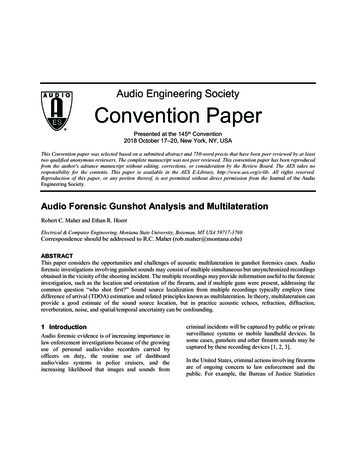
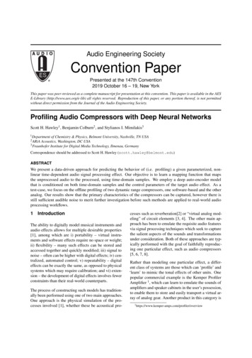
Hawley, Colburn, and MimilakisTypically audio effects are applied to an entire “stream”of data from beginning to end, yet it is not uncommonfor digital audio effects processors to be presented withonly a smaller “window” (also referred to as a “chunk,”“frame”, “input buffer,” etc.) of the most recent audio, of a duration usually determined by computationalrequirements such as memory and/or latency. For timedependent effects such as compressors, the size of thewindow can have repercussions as information preceding the window boundary will necessarily propagateinto the window currently under consideration. Thisintroduces a concern over “causality,” occurring overa timescale given by the exponential decay due to thecompressor’s attack and release controls.This suggests two different ways to approach training,and two different ways to specify the dataset of pairsof input audio and target output audio. The first werefer to as “streamed target” (ST) data, which is theusual method of applying the audio effect to the entirestream at once. The second we refer to “windowedtarget” (WT) data, in which the effect is applied sequentially to individual windows of input. WT datawill necessarily contain transient errors (compared toST data) occurring on a frequency of the inverse ofthe window duration. If however one adds a “lookbackbuffer,” i.e. making the length of the output shorter thanthat of the input, then this “lookback” can be chosen4 Thesystem could be modified to predict one sample at a time,however our experience with this model has found this practice to beneither necessary nor helpful.The difference between ST and WT data constitutes alower bound on the error produced by our neural network model: we do not expect the model to performbetter than the “true” effect applied to WT data. The dependence of this error bound on the size of the lookbackbuffer can be estimated in a straightforward way, andcan provide guidance on the size of buffer that shouldbe used when training the model. Such estimates areshown in Figure 1. In order to allow for low enougherror while not putting too great a strain on computational resources, we will choose model sizes withlookback windows sufficient to allow a lower bound onthe error in the range of 10 5 to 10 4 .Lookback (x103 samples)0481210 1Comp-4C10 210 410 62048819210 80.0Fig. 1:2.2Lookback (x103 samples)0100200Comp-4C-Large10 2MAEWe trained against two software compressors, with similar controls but different time scales. The effect wedesignate “Comp-4C” which operates in a sequentialmanner (later samples explicitly depend on earlier samples) and has four controls for Threshold, Ratio, Attackand Release. The other formulation, “Comp-4C-Large,”allows for wider ranges of the control parameters. Foran analog effect we used a Universal Audio LA-2A,output audio for a wide range of input audio as we varied the Peak Reduction knob and the Comp/Lim switch.(The input and output gain knobs were left fixed in thecreation of the dataset.) These effects are summarizedin Table 1.to be large enough that transient errors in the WT datadecay (exponentially) below the “noise floor” beforethe output is generated. The goal of this study is toproduce ST data as accurately as possible, as it corresponds to the normal application of audio effects, butWT data is in some sense “easier” to learn. Indeed, inour early attempts with the LA-2A compressor and STdata, the model was not able to learn at all, because thelookback buffer was not long enough.MAErange of inputs to a range of outputs, i.e., we windowthe audio into “windows.” This allows for both speedin computation as well as the potential for modelingnon-causal behavior such as reverse-audio effects ortime-alignment. 4Profiling Compressors with Deep Neural Nets0.2Lookback (s)10 310 42048819210 502Lookback (s)4Mean Absolute Error (MAE) betweenstreamed target (ST) data and windowed target(WT) data, for the software effect as a functionof lookback buffer size at 44.1 kHz, for twodifferent input window sizes (2048 and 8192).This represents a theoretical limit for the accuracy of the neural network model.Model SpecificationThe architecture of the SignalTrain model consists ofthe front-end, the autoencoder-like module, and theback-end module. The proposed architecture sharessome similarities with the U-Net [28] and TFNet [29]architectures. Like U-Net, it has an encoder-decoder“hourglass” configuration with skip connections spanning across the middle, and like TFNet, it operatesin both the time and spectral domains explicitly. TheAES 147th Convention, New York, 2019 October 16 – 19Page 3 of 11
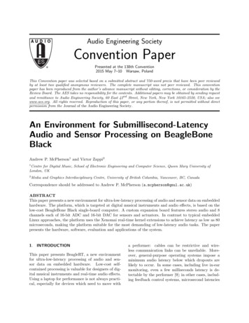
Hawley, Colburn, and MimilakisEffect nalogProfiling Compressors with Deep Neural NetsControls: RangesThreshold: -30–0 dB, Ratio: 1–5, Attack: 1–40 ms, Release: 1–40 msThreshold:-50–0 dB, Ratio: 1.5–10, Attack: 0.001-1 s, Release: 0.001-1 sComp/Lim Switch: 0/1, Peak Reduction: 0–100Table 1: Compressor effects trained. Comp-4C and Comp-4C-Large allow different control ranges but use thesame Python code, which is available in supplementary materials [26].front-end module is comprised by a set of two 1-Dconvolution operators that are responsible for producing a signal sub-space similar to a time-frequency decomposition, yielding magnitude and phase features.The autoencoder module consists of two deep neuralnetworks for processing individually the magnitudeand phase information of the front-end module. Eachdeep neural network in this autoencoder consists of 7fully connected, feed-forward neural networks (FC). Itshould be noted that the “bottleneck” latent space ofeach deep neural network is additionally conditionedon the control variables of the audio effect module thatare represented as one-hot encoded vectors.Figure 2 illustrates the neural network architecture forthe SignalTrain model, which essentially learns a mapping function from the un-processed to the processedaudio, by the audio effect to be profiled, and is conditioned on the vector of the effect’s controls (e.g., the“knobs”). In order to obtain the predicted output waveform, the back-end module uses another set of two 1-Dtransposed convolutional operators. Similarly to theanalysis front-end, the back-end is initialized using thebases of a discrete Fourier transform. It should be statedthat all the weights are subject to optimization and areexpected to vary during the training of the model. Theframe and hop sizes used for the convolutions are 1024and 384 samples, respectively.Unlike some other proposed architectures which useconvolutional layers [28], we use fully-connected (FC)layers that have shared-weights with respect to the subspace dimensionality (i.e., the frequencies). That isdone for two reasons. The first reason is that the number of the parameters inside the model is dramaticallyreduced, and secondly we preserve the location of themagnitude and phase information of the original signal.Essentially, the operations carried by each deep neural network in the autoencoder module can be seen asnon-linear affine transformations of the transpose timefrequency patches (spectrograms) of the input signal.Furthermore, we apply residual (additive) skip connections [31] inspired by U-Net [28] and “skip filter”Fig. 2: Diagram of the SignalTrain network architecture. The designations ‘STFT,’ ‘ISTFT,’ ‘Magnitude’ and ‘Phase’ are used for simplicity,since the complex-valued discrete Fourier transform is used to initialize the weights of the1-D convolution layers. All other layers arefully-connected (FC) with ELU [30] activations.Typically our output and target waveforms aresmaller than the input; this difference in size(indicated by the cross-hatched region designated “lookback”) means the autoencoder is‘asymmetric.’ On the autoencoder output, the“magnitude spectrogram designated M̃ is usedfor regularizing the loss, Eq. (1).(multiplicative) connection for the magnitude only [19].These skip connections dramatically improve the speedof training, and can be viewed in three complementary ways: allowing information to propagate furtherthrough the network, smoothing the loss surface [32],and/or allowing the network to compute formidableperturbations subject to the goal of profiling an audioeffect.AES 147th Convention, New York, 2019 October 16 – 19Page 4 of 11
Hawley, Colburn, and MimilakisIn the middle of the autoencoder, we concatenate valuesof the effect controls (e.g., threshold, ratio, etc.) and“merge” these via an additional FC layer. The first layerof the autoencoder maps the number of time frames inthe spectrograms to 64, with subsequent layers shrinking (or, on the output side, growing) this by factors of2. The resulting model has approximately 4 milliontrainable parameters.2.3Training ProcedureWe use a log-cosh loss function [33], which has similarproperties to the MAE (i.e., L1 norm divided by thenumber of elements) in the sense that it forces thepredicted signal to closely follow the target signal at alltimes, however the roundness of the log-cosh functionnear zero allows for significantly better training at lowloss values than does L1, which has a discontinuousderivative at zero.Furthermore we include an L1 regularization term witha small coefficient λ (e.g., 2e-5), consisting of the magnitude spectrogram M̃ from the output side of the autoencoder, weighted exponentially by frequency-binnumber fk to help reduce high-frequency noise in thepredicted output. Thus the equation for the loss function is given byLoss log [cosh (ỹ y)] λ exp[( fk ) α ] · M̃ L1 , (1)where ỹ and y are the predicted and target outputs,respectively, and choosing α 1 implies exponentialweighting by frequency bin fk , and choosing α 0disables any such weighting.Simply training on a large amount of musical audiofiles is not necessarily the most efficient way to trainthe network – depending on the type of effect beingprofiled, some signals may be more ‘instructive’ thanothers. A compressor requires numerous transients ofsignificant size, whereas an echo (or ‘delay’) effect maytrain most efficiently on uncorrelated input signals (e.g.,white or pink noise). Therefore, we augment a datasetof music recordings with randomly-generated soundsintended to provide both dynamic range variation andbroadband frequency coverage.By virtue of the automation afforded by software effects such as Comp-4C, we can train indefinitely using randomly-synthesized signals which change during each iteration. But for the LA-2A, we created alarge (20 GB) input dataset of public domain musicalProfiling Compressors with Deep Neural Netssounds and randomly-generated test sounds, concatenated these and divided the result into (unique) files of15-minute duration, using a fixed increment of “5" onthe LA-2A’s Peak Reduction knob between recordings,for both settings of the Comp/Lim switch. For prerecorded (i.e., non-synthesized) audio, windows from theinput (and for ST data, target) data are copied from random locations in the audio files, along with the controlsettings used. Data augmentation is applied only inthe form of randomly flipping the phase of inputs andtargets.To achieve the results in this paper, we trained fortwo days (see “Implementation,” below) on what corresponded to approximately 2000 hours of audio sampledat 44.1 kHz (or 130 GB if it were stored on disk). Asa performance metric, we keep a separate, fixed “validation set” of approximately 12 minutes of audio; allresults displayed in this paper are for validation data,i.e., on data which the network has not “seen” before.The arrangement of this data is “maximally shuffled,”i.e., we find that training is significantly more smoothand stable when the control settings are randomlychanged for each data window within each mini-batch.Trying to train using the same knob settings for large sequences of inputs – as one might expect to do by takinga lengthy pair of (input-output) audio clips obtained atone effect setting and breaking them up into a sequential mini-batch of training windows – results in unstabletraining in the sense that the (training and/or validation) loss varies much more erratically and, overall,decreases much more slowly than for the ‘maximallyshuffled’ case in which one varies the knob settingswith every window. This shuffling from window towindow is another reason why our model is not autoregressive: because we wish to learn to model thecontrols with the effect.When starting from scratch, weights are initialized randomly except for the weights connecting to the inputand output layers convolutional layers, which are initialized using basis values corresponding to a DiscreteFourier Transform (DFT), and its inverse transform,respectively. These are subsequently allowed to evolveas training proceeds. For the different task of imageclassification on the ImageNet dataset [34], the combination of Adam [35] with weight decay [36] has beenshown [37] to be among the fastest training methodsavailable when combined with learning rate scheduling.We also adopt this combination for our problem.AES 147th Convention, New York, 2019 October 16 – 19Page 5 of 11
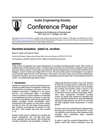
Hawley, Colburn, and MimilakisAn important feature, found to decrease both final validation loss values and the number of epochs requiredto reach them, is the use of learning rate scheduling,i.e., adjusting the value of the learning rate dynamically during the course of gradient-based optimization,rather than keeping the learning rate static. We followthe “1-cycle” policy [38], which incorporates cosine annealing [39], in the manner popularized by the Fasti.aiteam [40]. Compared to using a static learning rate, the1-cycle policy allowed us to reach roughly 1/10th theerror in 1/5 the time.Implementation3.1Software Compressor: “Comp-4C”We ported MATLAB code to Python for a single-band,hard-knee compressor with four controls: threshold,ratio, attack and release times [42]. (This compressorimplements no side-chaining, make-up gain or otherfeatures.) As it is a software compressor, the trainingdata could be generated “on the fly," choosing control(‘knob’) settings randomly according to some probability distribution (e.g., uniform, or a beta distributionto emphasize the endpoints 6 ). This synthesis allowsfor a virtually limitless size of the training dataset. Ourearly experiments used such a dataset, but given thatintended goal of this system is to profile systems withina finite amount of time, and particularly analog effectswhich would typically require the creation of a finiteset of recordings, we chose to emulate the intended usecase for analog gear, namely a finite dataset in whichthe control knob settings are equally spaced, with 10settings per control.5 https://github.com/NVIDIA/apex6 Initially we chose control settings according to a symmetric betadistribution, with the idea that by mildly emphasizing the endpointsof the control ranges, the model would learn more efficiently, however experience showed no performance enhancement compared tochoosing from a uniform distribution.T -2 dBResultsInputA/R 0.005 s0.5T -12 dBThe SignalTrain code was written in Python using thePyTorch [41] library along with Numba for speedingup certain subroutines. Development and training wasprimarily conducted on a desktop computer with twoNVIDIA Titan X GPUs. Later in the project we upgraded to two RTX 2080Ti GPUs, which, with the benefit of NVIDIA’s “Apex” mixed-precision (MP) traininglibrary 5 , yielded speedup of 1.8x over the earlier runs.3Figure 3 shows the performance of the model comparedto the target audio, for the case of a step-response, acommon diagnostic signal for compressor performance[4, 8, 43]. The predicted values follow the target closelyenough that we show their differences in Figure 4. Keydifferences occur at the discontinuities themselves (especially at low attack times), and we see that the predictions tend to “overshoot” slightly on at the releasediscontinuity (we speculate that this is due to slighterrors in the phase in the spectral decomposition in themodel), but that in between and after the discontinuitiesthe predictions and target match closely.0.5T -24 dB2.4Profiling Compressors with Deep Neural Nets0.5TargetA/R 0.015 sPredictedA/R 0.03 s0.00.00.00.000 0.025 0.050 0.075 0.000 0.025 0.050 0.075 0.000 0.025 0.050 0.075t (s)t (s)t (s)Fig. 3: Sample model step-response performance forthe Comp-4C effect using WT data on a domainof 4096 samples at 44.1 kHz, for various valuesof threshold (T) and attack-release (A/R, setequivalently). In all graphs, the ratio 3. SeeFigure 4 for a plot of the difference betweenpredicted and target outputs, and SupplementalMaterials [26] for audio samples and an interactive demo with various input waveforms andadjustable parameters.As noted in Section 2.1, the size of the lookback window can have an effect on the error bounds. Figure 5shows that the loss on the Validation set to be consistentwith estimates obtained for the cases depicted in Figure1. And yet listening to these examples (see Supplemental Materials [26]) one notices noise in the predictedresults, suggesting that the lookback window size (or“causality noise”) is not the only source of error in themodel.Although step responses are a useful diagnostic, theneural network model approximates the input-outputmappings it is trained on, and is ultimately intendedAES 147th Convention, New York, 2019 October 16 – 19Page 6 of 11
Hawley, Colburn, and MimilakisA/R 0.005 sT -2 dB0.2Profiling Compressors with Deep Neural NetsDifference Target-PredictedA/R 0.015 s 20A/R 0.03 s0.1 300.0 40Level (dB)T -12 dB0.20.10.0T -24 dB0.2 50 600.1 700.00.000.05t (s)0.000.05t (s)0.00 800.05t (s)101Fig. 4: The difference between predicted and targetoutputs for the step responses shown in Figure3. We see the largest errors occur precisely atthe step discontinuities, likely due to inadequateapproximation in the “spectral” representationwithin the model.LossTraining102103104ValidationST 92.9msWT 92.9msST 2.88sWT 2.88s100101102Epoch103 100101102Epoch103Fig. 5: Typical loss on Training & Validation sets forComp-4C-Large effect, while training for STand WT data, for two different lookback window lengths. (Because our data is randomlysampled, “Epoch” does not refer to a completepass through the dataset, but rather the arbitraryselection of 1000 mini-batches.)for use with musical sounds which may typically lacksuch sharp discontinuities. Thus a comparison of compressor output for musical sounds is in order as well.Figure 6 shows a comparison of frequency spectrumfor a full-band recording (i.e., drums, bass, guitar, vocals) in the testing dataset. It also shows that scalingthe L1 regularization exponentially by frequency canyield a reduction in high-frequency noise, sacrificingTargetPredicted, α 0Predicted, α 1102103Frequency (Hz)104Fig. 6: Power spectra for musical audio in the Testdataset [26] compressed with Comp-4C controlparameters [-30, 2.5, .002, .03]. Here we seethe effects of weighting the L1 regularizationin the loss function Eq. (1) exponentially byfrequency (α 1) or not (α 0): weightingby frequency shifts a nontrivial amount of highfrequency noise toward a proportionally smallincrease at low frequencies. Although noise isstill clearly audible in both predicted outputs(refer to Supplemental Materials [26] to hearaudio samples), the result is that the listener perceives less overall noise in the output when thefrequency-weighted L1 regularization is used.a proportionally smaller amount of accuracy at lowfrequencies.3.2Analog Compressor: LA-2AA primary interest in the application our method is notfor cases in which a software plugin already exists, butrather for the profiling of analog units. As an example,we choose the Universal Audio’s Teletronix LA-2A, anelectro-optical compressor-limiter [44], the controls forwhich consist of three knobs and one switch. Giventhat two of the knobs are only for input-output gainadjustment, for this study, we focus only on varying the“Peak Reduction” (PR) knob, and the “Compress/Limit”switch. The switch is treated like a knob, with limits of0 for “Compress" to 1 for “Limit."Figure 7 shows the loss on the validation set for theLA-2A for different lookback sizes. The dashed (black)line shows a model with an input size of 8192*2 16384AES 147th Convention, New York, 2019 October 16 – 19Page 7 of 11
Hawley, Colburn, and MimilakisProfiling Compressors with Deep Neural Nets10 3100101102103EpochFig. 7: Training history on the LA-2A dataset for different lookback sizes. The “kink” near epoch300 is a common feature of the 1-cycle policy [38, 40] when using an “aggressive” learning rate (in this case, 7e-4). Both runs achievecomparable losses despite the longer lookbackbuffer needing nearly 5 times as much execution time.and took 15 hours to run, the solid (blue) line is a modelwith input size of 8192*27 221184 and took 72 hours.Both runs used output sizes of 8192 samples. In all ourruns, a loss value of approximately 1e-4 is achieved, regardless of the size of the model – even for a lookbackextending beyond the “5 seconds for complete release”typically associated with the LA-2A [45]. This indicates that the finite size of the lookback window (or“causality noise”) is not the primary source of error;this is consistent with the Comp-4C results (e.g., seeFigure 5). The primary source of error remains anongoing subject of investigation. Graphs of exampleaudio waveforms from the Testing dataset are shown inFigure 8, where it is noteworthy that the model will attimes over-compress the onset of an attack as comparedto the true LA2A target response.ConclusionIn pursuit of the goal of capturing and modeling genericaudio effects by means of artificial
linear time-dependent audio signal processing effect. Our objective is to learn a mapping function that maps the unprocessed audio to the processed, using time-domain samples. We employ a deep auto-encoder model that is conditioned on both time-domain samples and the control parameters of the target audio effect. As a