Transcription
Page 1Intermediate Microsoft Excel 2010ABOUT THIS CLASSThis class is designed to continue where the Microsoft Excel 2010 Basics class left off. Specifically, we will coveradditional ways to organize data as well as how to create different types of charts. It is impossible in these two hours tobecome totally proficient using Microsoft Excel, but it is my hope that this class will provide added skills to furtherlaunch you into this exciting world!Course ObjectivesBy the end of this course, you will be able to Manage multiple workbooks. Freeze panes. Sort and filter data. Use the Text-to-Columns feature to organize data from single to multiple cells. Create basic charts (clustered column, pie, etc.). Create PivotTables and PivotCharts.This booklet will serve as a guide as we progress through the class, but it can also be a valuable tool when you areworking on your own. Any class instruction is only as effective as the time and effort you are willing to invest in it. Iencourage you to practice soon after class. There will be additional computer classes in the near future, and I am alwaysavailable for questions during Tech Tuesdays (call to confirm the time).Cody Yantis, Technology Services Librarian
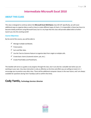
Page 2Managing WorkbooksIn Excel Basics, we learned how to manage multiple worksheets. Let’s look at how to manage multiple workbooks. Exceluses the term workbook for a file. The term worksheet refers to an individual spreadsheet within a workbook. Aworkbook can contain multiple worksheets, each have their own tab. It is possible to have multiple workbooks (.xlsxfiles) open concurrently.Switching Between Open Workbooks1. Open Excel and create two additional new workbooks. To create a new workbook click File New BlankWorkbook.2. Save the workbooks. Let’s name them: This, That, and The Other.3. Select the View tab Window group Switch Windows.4. In the menu that appears, you will see a listing of the workbooks that are open.5. Click the file that you want to bring to the foreground. The file that was in the foreground remains open, but isnow in the background.View Multiple Open Workbooks1. Select View tab Window group Arrange All.2. Select Tiled and click OK.All three windows are now arranged in such a way that you can view and edit them all at once:
Page 3Freezing PanesWhile we’re in the View tab, let’s learn how to freeze panes. When working with large or complex worksheets, scrollingcan sometimes become a problem. Freezing panes allows you to keep specific rows and/or columns visible as you scroll.To enable this option: Select View tab Window group Freeze PanesYou can then select which panes you wish to freeze: all cells (freeze panes), the top row (freeze top row), or the firstcolumn (freeze first column).To turn off this option: Select View tab Windows group Freeze Panes Unfreeze PanesOrganize that Data! Using the Data TabSortingInformation can be sorted into alphabetical or numerical order, ascending or descending. Excel can change the rownumbers that related information appears in while also keeping items together.Exercise 1. Sorting by multiple levels1. Open the workbook on your desktop titled Sorting and Filtering.2. Highlight the entire data selection (A1:C7).3. Click Data tab Sort & Filter Sort.4. Make sure that My data has headers is checked (it should be, as that’s the default).5. Select Last in the Sort by drop down menu.6. Click Add Level.7. Select First in the Then by drop down menu.8. Click Add level.9. Select Title in the second Then by drop down menu.
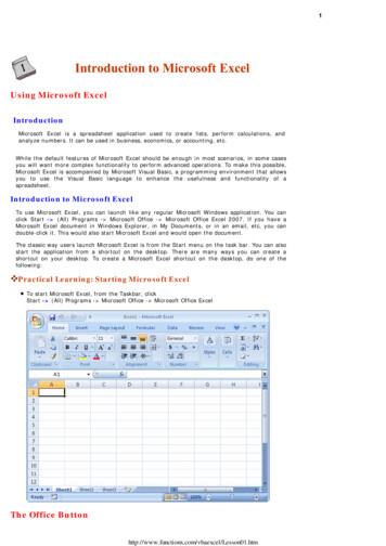
Page 410. Click OK.The entire selection will then sort by your parameters.Tip: If you have data in multiple and corresponding columns but only highlight one column and click Sort, Excel will askyou if you want to expand your sort to include the entire selection. This helps to avoid sorting one column but notanother, which often results in skewed data.FilteringYou can filter to select records that match specific criteria. This gives a temporary view of data without physicallyremoving anything. Let’s filter our list of names by title so that only the Ms. entries are listed.Exercise 2. Filtering1. In the Sorting and Filtering workbook, highlight the entire data selection (A1:C7).2. Click Data tab Sort & Filter Filter. Notice that down arrow buttons appear above each column.3. Click on the down arrow button above the Title column.4. Uncheck the box next to Mr.5. Click OK.Notice that only the Ms. entries are now displayed:
Page 5To unfilter, click Data tab Sort & Filter Filter.Tip: Notice in the above screenshot, that the cell numbers are not ordered. This is an indication that, when filtering, youare not deleting data, but merely hiding data (in this case, all of the Mr. entries).Text to ColumnsIf you have entered or copied some text into a single column, you can use the Text to Columns command to portion itout into adjacent columns (make sure these columns are blank before proceeding).Exercise 3. Text to Columns (Space Delimiting)1. Open the Text to Columns workbook on your desktop.2. Notice that Column A has first and last names in each cell. We’re going to split the first and last names intodifferent cells and columns.3. Highlight Column A.4. Click Data tab Data Tools Text to Columns.5. Select Delimited and click Next.6. Check Space. Notice that a preview of your data is displayed below. Click Next.7. The data is already formatted in terms of data type, so then click Finish.Notice that your first and last names are now split into different columns!Exercise 4. Text to Columns (Comma Delimiting)1. Notice that Column D has last then first names separated by a comma in each cell. We’re going to split the firstand last names into different cells.2. Highlight Column D.3. Click Data tab Data Tools Text to Columns.4. Select Delimited and click Next.5. Check Comma. Notice that a preview of your data is displayed below. Click Next.6. The data is already formatted in terms of data type, so then click Finish.Notice that, again, your first and last names are now split into different columns!Tip: to remove that unwanted space in front of the first name from our comma delimited group:1.2.3.4.Highlight the column.Click Ctrl-H (“Find and Replace”).In the Find What field, enter a space.Leave Replace With field blank and click OK.
Page 6The spaces are removed! You can use Ctrl-H to find any type of data and replace it with something (or nothing) else!(Added Tip: The Clean and Trim functions will perform a similar task, in addition to removing other unnecessary data[html, etc.].)ChartsThere are numerous ways to render data visually into charts. In general, if you have organized your data in a way thatcan be easily interpreted by Excel, the program can automatically convert this data into a chart. Let’s start by creating abasic Clustered Column chart.Exercise 5. Creating a Clustered Column Chart1. Open the Chart Data workbook on your desktop.2. Notice that there are two points of data (type and number of animals), which have been organized into rowsand columns:3. Highlight the entire data selection (A1:E2).4. Click Insert Tab Charts Create Chart:5. Select Clustered Column and then click OK:
Page 7A basic clustered column will then display:Formatting Tips:1. You can change the chart style by clicking on the chart and then: Chart Tools Design Tab Chart Styles andthen selecting a different style.2. You can change the chart type by clicking on the chart and then: Chart Tools Design Tab Type and selecting adifferent chart type (for instance, a pie or a line chart). If you find a chart type that you really like, you can set itas your default: Click: Chart Tools Design Tab Type. Select the chart type. Click on Set as Default Chart.PivotTables & PivotChartsWhen you have multiple or fluid data categories and/or when you have data that hasn’t already been organized, theeasiest way to turn this into a chart is to create a PivotTable, which can then be quickly converted into a PivotChart. APivotTable interactively allows for quickly summarizing large amounts of data. You can rotate its rows and columns tosee different summaries of the source data, filter the data by displaying different pages, or display the details for areasof interest. PivotCharts are associated with PivotTables and provide graphical representations of the same information.Use a PivotTable when you want to compare related totals, especially when you have a long list of figures to summarizeand you want to compare several facts about each figure. Because a PivotTable is interactive, you can change the viewof the data to see more details or calculate different summaries. This gives a customized perspective on the datawithout having to change anything in the range of cells it is based on.
Page 8Exercise 6. Creating a PivotTable & PivotChartIn this exercise, we will take raw data based on four agents at an insurance company and look at their sales over thecourse of a year for three different product types. The existing data was entered in such a way that it is somewhatredundant and hard to draw conclusions from readily. By placing it into a PivotTable with an associated chart, we caneasily streamline this into useful information and quickly manipulate it into multiple views to help us draw conclusions.1. Open the Pivot Data workbook on your desktop.2. Select the range that encompasses the headings and data (A1:D26).3. Select Insert tab Tables PivotTable drop-down PivotChart:4. Confirm that you accurately selected the correct data by clicking OK.5. The Pivot Table Field List box will then appear. This is how you determine which data is displayed in which fieldin the PivotTable.6. Check all four fields to add to report.7. Then drag:a. Quarter to: Report Filter.b. Type to: Legend Fields.c. Agent to: Axis Fields.d. Amount to: Values Field. (Tip: Excel deduces that this is where you will want Amount, since it’s the lastremaining field. Thus, you may not need to move it.)
Page 9You will then have a PivotTable and PivotChart that has organized and displayed the information based on the criteriawe selected:
P a g e 10Editing Your PivotTable & ChartBelow are some tips for editing your PivotTable and PivotChart:1. To rearrange the chart’s orientation on the spreadsheet, just click and drag it.2. Edit the appearance and style of the chart by clicking on the Pivot Chart and then selecting from different chartstyles (PivotChart Tools Design tab Chart Styles):3. You can edit the PivotChart parameters at any time by clicking on the PivotChart (at which point the Pivot TableField List will reappear).4. You can also reorganize the data via the dropdown menus above the data columns and on the PivotTable. Thisis the interactive element of the PivotTable (putting the “pivot” in PivotTable!).a. For instance, all quarters (First through Fourth) are currently displayed. If you wish to view the data byquarter, click on the down arrow menu labeled Quarter on the table or chart, and select the quarter youwish to view. You can do the same for each agent.Congratulations! You’ve completed the Intermediate MS Excel 2010 class. Please take a moment to fill out thisonline survey. Your feedback is very important to the /
Excel uses the term workbook for a file. The term worksheet refers to an individual spreadsheet within a workbook. A workbook can contain multiple worksheets, each have their own tab. It is possible to have multiple workbooks (.xlsx files) open concurrently. Switching Between Open Workbooks 1. Open Excel and create two additional new workbooks.