WIXLIB

International Journal of Engineering Research & Technology (IJERT)ISSN: 2278-0181Vol. 4 Issue 03, March-2015Modeling and Forecasting by using Time SeriesARIMA ModelsMustafa M. Ali AlfakiDr. (Ms.) Shalini Bhawana MasihResearch Scholar,School of Basic ScienceSam Higginbottom Institute of Agriculture,Technology and SciencesAllahabad, IndiaAssistant Professor,School of Basic ScienceSam Higginbottom Institute of Agriculture,Technology and SciencesAllahabad, IndiaAbstract:-- In this paper we introduce a brief review aboutBox-Jenkins models. “Auto-Regressive Integrated MovingAverage”, Known as ARIMA models. It is a good method toforecast for stationary and non stationary time series.According to the data which obtained from the monthly salesfor Naphtha product in Azzawiya Oil Refining Company –Libya, then we determine an optimal model. The results ofthis study showed that the suitable and efficient model torepresent the data of the time series according to AIC, SIC,and MSE criteria with the smallest values as well as the Boxljung test is the ARIMA(1,1,1), whose equation is :Zˆt 0.6010 Z t 1 1.1713 εt 1 ε tAccording to the results of ARIMA (1,1,1), the amounts of themonthly sales for Naphtha product Azzawiya Oil RefiningCompany – Libya, have been forecasted for the period fromJan: 2015 to Dec: 2020. Those values showed harmony withtheir counterparts in the original time series. It provided uswith a future image of the reality of the monthly sales forNaphtha product in Azzawiya Oil Refining Company – Libya.Key Words : Forecasting, Box-Jenkins, Auto-RegressiveIntegrated Moving Average (ARIMA), Auto-Regressive (AR),Moving Average (MA), Autocorrelation Function (ACF),Partial Autocorrelation Function (PACF).appropriate model for this time series. This model is theassessed to determine how well it’s the data.Non-seasonal Box-Jenkins Models for a Stationary Series:That is known as (ARIMA) Models, it is an AutoregressiveModel AR(p) as the first part, and Moving Average ModelMA(q) a second part, and the third part I(d) represents thedifferences required by the time-series in order to bestationary. Some models of time series may be nonstationary of the same kind but they would becomeStationary after a lot of differences and changes, so that themodel which represents this process will vary from theoriginal model because it will include those differences andchanges made by the model by taking appropriate numberof operational differences process.Autoregressive Models AR(p):Which has the general form:Z t 1 Z t 1 2 Z t 2 . p Z t p t,t p(1)Where :Z t dependent variable at time t.INTRODUCTIONThe planning process is the most important step in thedevelop plan of any country, it becomes adequate if thestatistical methods that has been applied are based onpowerful scientific basis.The time series is a set of well-defined data items collectedat successive points at uniform time intervals. Time seriesanalysis is an important part in statistics, which analyzesdata set to study the characteristics of the data and helps inpredicting future values of the series based on thecharacteristics. Forecasting is important in fields likefinance, industry, etc. The Autoregressive IntegratedMoving Average (ARIMA) is based on ARMA Model. Thedifference is that ARIMA Modelconverts a non-stationarydata to a stationary data before working on it. This analysisuses Box-Jenkins ARIMA modeling techniques to find anIJERTV4IS030817Z t 1 , Z t 2 , , Z t p dependent variable at time lags t 1, t 2, . . . , t p respectively. i :Coefficients to be estimated, as:i 1 , 2 , 3 , . p , t : 1 P 1Series of random errors, with mean zero and constantvariance. i . e . t N (0, 2 ) .Moving Average Model MA (q):Which has the general form: t t 1 t 1 2 t 2 . q t q(2)Where:Z t dependent variable at time t.www.ijert.org(This work is licensed under a Creative Commons Attribution 4.0 International License.)914

International Journal of Engineering Research & Technology (IJERT)ISSN: 2278-0181Vol. 4 Issue 03, March-2015 t :Series of random errors, with mean zero and constantvariance. i . e . t 1 t N (0, 2 ) ., t 1 , . t q Errors in previous time periodsthat are incorporated in the response Z t . i: Parameters of moving average model.q : Degree Model.Mixed Models ARMA ( p , q ):Which has the general form:Figure (1): Graphical representation of the series Naphtha t 1 t 1 2 t 2 . p t p t 1 t 1 . q t qTable (1): ACF and PACF of the series NaphthaAutoregressive Integrated Moving Average ModelARIMA (p,d,q):The general formula of Autoregressive Integrated MovingAverage Models (ARIMA) That is written as : t 1 t 1 2 t 2 . p t p . d t p d t 1 t 1 . q t q(4)Building ARIMA Model and Forecasting:The data used in this study consist of the monthly sales forNaphtha production in Azzawiya Oil Refining Company –Libya, for the period (2008 – 2014).StationaryIn order to apply certain techniques for identifying andARIMA model for the data, we must determine the form ofstationary of the original time series and we will draw theautocorrelation function (ACF), and the partialautocorrelation function (PACF) of data and drawconfidence interval of (ACF) and (PACF) to detect thestationary or non-stationary of time series, as well as theuse of the Q test, (Box- Ljung test) where:mQ m n (n 2)ρ̂2k n k 2(m)Q 245.99 (5)k 12 25, 0.05 37.652And to make the series stationary we make differencesfrom First level while taking the natural logarithm of thedata and then we can obtain the following results:Where:ρ̂ kThrough the Figure (1) and table (1) of the original seriesof Correlation Coefficients and figures of ACF and PACF,we note that there is non- stationary in the data of originalseries as there are some values outside the confidenceinterval, and that the significant value of the Coefficientsautocorrelation function using the Q test : the residual autocorrelation at lag k.n the number of residuals.m the number of time lags includes in the test.And we will test of unit root by Augmented Dickey-Fuller(ADF) test on the original data provided evidence of thepresence of a unit root we difference the data to counteractthe effect of this unit root. We depended on Eviews.5program to determine tables and figures we can obtain thefollowing results:IJERTV4IS030817www.ijert.org(This work is licensed under a Creative Commons Attribution 4.0 International License.)915

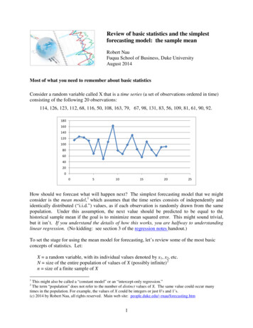
International Journal of Engineering Research & Technology (IJERT)ISSN: 2278-0181Vol. 4 Issue 03, March-2015Table (3): ADF test results for series D(Log(Naphtha))Through the data of the table (3) we note that all calculatedstatistics of Dickey Fuller in all models are less than thecorresponding tabular values, then there is no a unit root inthe series, and the series D(Log(Naphtha)) is stationary.Figure (2): Graphical representation of the series D(Log(Naphtha))Table (2): ACF and PACF of the series D (log(Naphtha))Model Identification:Through the table (2), we observe the presence of movingaverages models MA (1), MA (3) and MA (6), throughthe autocorrelation function. And the presence ofautoregressive models AR (1), AR (3) andAR (6),through partial autocorrelation function, and for moreaccuracy in reconciling the best model among Box-Jenkinsmodels, possible models of ARIMA (p, d, q) have beenapplied, and calculation of each of them SC, AIC and MSEare as shown in the following table:Table (4): Compared to a set of valuesof AIC , SIC , MSEFrom the table (4), we find that the model ARIMA (1,1,1)is the one who gives the lower values of the previousstandards, these values were as follows:MSE 0.3506 , AIC 1.8629 , SC 1.9510So this model was relied on to be an appropriate model forthis series.Through the figure (2) and table (2) of modified series ofcorrelation coefficients and figures of ACF and PACF wenote that there is stationary in the data of series and most ofthe values within the confidence interval, and that theSignificant value of autocorrelation coefficients by usingthe Q test was:Q 13.586 2 25, 0.05 37.652We then test by Advanced Dickey Fuller and the estimationof models is as follows:IJERTV4IS030817Model Diagnostics:Residual diagnostic tests and the over fitting process areused here to determine the goodness of fit of theARIMA(1,1,1) model to the original time series. Residual Diagnostics:We have been used diagnostic the ACF for the residuals.Here we see that the ACF values are all within the 95%,indicating that there is no correlation amongst the residuals.This plot is used as an indicator of the independence of theresidual.www.ijert.org(This work is licensed under a Creative Commons Attribution 4.0 International License.)916

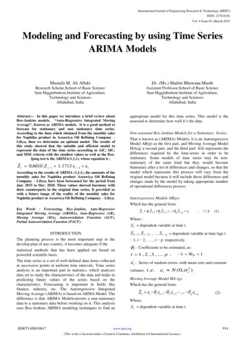
International Journal of Engineering Research & Technology (IJERT)ISSN: 2278-0181Vol. 4 Issue 03, March-2015Table (5): ACF and PACF for Residual ARIMA (1,1,1)analyzed ( Naphtha product). The final model is of thefollowing form:Table (6): Estimated model parameters of Naphtha salesmodelWe obtained the model in the form:Zˆ t 0.6010 Z t 1 1.1713 ε t 1 ε tFrom the table (5) we note that the most of the coefficientsfall within the confidence interval, as well as the statistical(Q): 225, 0.05Q 10 (6)ForecastingAfter the identification of the model and its adequacycheck, it is used to forecast the sales for Naphtha product inAzzawiya Oil Refining Company – Libya in the period(January 2015 to December 2020). The forecasting resultsare presented in figure (4)5.0E 12 37.6524.0E 12Therefore Residuals represent white noise.3.0E 12Normal distribution test:The residuals follow the normal distribution in thefollowing diagram:2.0E 121.0E 1232Series: ResidualsSample 2008M03 2014M12Observations 82280.0E 00201524MeanMedianMaximumMinimumStd. 0-0.50.00.51.01.5Figure (3): Testing of normal distribution of residuals seriesThe distribution of residuals are almost symmetrical.Autocorrelation test for errors (Durbin-Watson's statistic):The value of D-W 1.9924, it is lies within theconfidence interval, hence it has no Auto correlation oferrors. Then all the results of the residuals tests confirm thevalidity of the estimated model ARIMA (1,1,1) to representthe time series.20192020CONCLUSIONThe aim of this analysis was to determine an appropriateARIMA model for the sales Monthly data for Naphthaproduct. In particular we were interested in forecastingfuture for sales of company using this model. It isconcluded that the ARIMA (1,1,1), where were the valueof MSE, AIC and SC for the model are very small. Hencethe model is appropriate to forecast the sales of Naphthafor the next six years.REFERENCES1.Final ModelTherefore conclude that the ARIMA(1,1,1) modelis the best ARIMA model for the original time series beingIJERTV4IS0308172018Figure (4): Forecasted Naphtha SalesJarque-Bera 353.5694Probability 0.000000-3.02017NAPHTF8420162.David A. Bessler. (1982). Adaptive Expectations. TheExponentially Weighted Forecast and Optimal StatisticalPredictors: A Revist. Agricultural Economics Research., 34 (2),pp, 16-23.Abraham, B. and Ledoter. J, (1983). “Statistcal Methods forForecasting” , John Wiley, New York.www.ijert.org(This work is licensed under a Creative Commons Attribution 4.0 International License.)917