WIXLIB

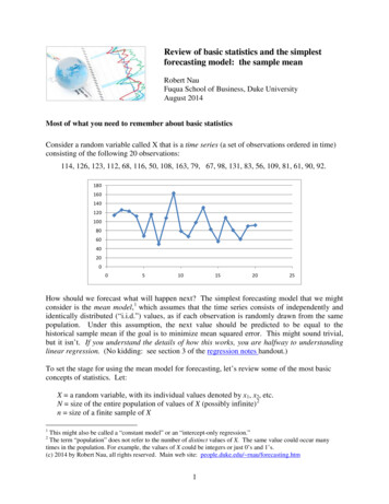
Review of basic statistics and the simplestforecasting model: the sample meanRobert NauFuqua School of Business, Duke UniversityAugust 2014Most of what you need to remember about basic statisticsConsider a random variable called X that is a time series (a set of observations ordered in time)consisting of the following 20 observations:114, 126, 123, 112, 68, 116, 50, 108, 163, 79, 67, 98, 131, 83, 56, 109, 81, 61, 90, 92.1801601401201008060402000510152025How should we forecast what will happen next? The simplest forecasting model that we mightconsider is the mean model, 1 which assumes that the time series consists of independently andidentically distributed (“i.i.d.”) values, as if each observation is randomly drawn from the samepopulation. Under this assumption, the next value should be predicted to be equal to thehistorical sample mean if the goal is to minimize mean squared error. This might sound trivial,but it isn’t. If you understand the details of how this works, you are halfway to understandinglinear regression. (No kidding: see section 3 of the regression notes handout.)To set the stage for using the mean model for forecasting, let’s review some of the most basicconcepts of statistics. Let:X a random variable, with its individual values denoted by x1, x2, etc.N size of the entire population of values of X (possibly infinite) 2n size of a finite sample of X1This might also be called a “constant model” or an “intercept-only regression.”The term “population” does not refer to the number of distinct values of X. The same value could occur manytimes in the population. For example, the values of X could be integers or just 0’s and 1’s.(c) 2014 by Robert Nau, all rights reserved. Main web site: people.duke.edu/ rnau/forecasting.htm21

The population (“true”) mean µ is the average of the all values in the population:µ iN 1 xi NThe population variance σ is the average squared deviation from the true mean:2( x µ )2 i 1 i Nσ2NThe population standard deviation σ is the square root of the population variance, i.e., the “rootmean squared” deviation from the true mean.In forecasting applications, we never observe the whole population. The problem is to forecastfrom a finite sample. Hence statistics such as means and standard deviations must be estimatedwith error.The sample mean is the average of the all values in the sample:X in 1 xi nThis is the “point forecast” of the mean model for all future values of the same variable. Thesample mean of the series X that was shown above is 96.35. So, under the assumptions of themean model, the point forecast for X for all future time periods should be 96.35.The sample variance s2 is the average squared deviation from the sample mean, except with afactor of n 1 rather than n in the denominator:( x X )2 i 1 i ns2n 1The sample standard deviation is the square root of the sample variance, denoted by s. Thesample standard deviation of the series X is equal to 28.96.Why the factor of n 1 in the denominator of the sample variance formula, rather than n? Thiscorrects for the fact that the mean has been estimated from the same sample, which “fudges” it ina direction that makes the mean squared deviation around it less than it ought to be. Technicallywe say that a “degree of freedom for error” has been used up by calculating the sample meanfrom the same data. The correct adjustment to get an “unbiased” estimate of the true variance isto divide the sum of squared deviations by the number of degrees of freedom, not the number ofdata points2

The corresponding statistical functions in Excel 3 are: Population mean AVERAGE (x1, xN) Population variance VAR.P (x1, xN) Population std. dev. STDEV.P (x1, xN) Sample mean AVERAGE (x1, xn) Sample variance VAR.S (x1, xn) Sample std. dev. STDEV.S (x1, xn)Now, why all this obsession with squared error? It is traditional in the field of statistics tomeasure variability in terms of average squared deviations instead of average absolute 4deviations around a central value, because squared error has a lot of nice properties: The central value around which the sum of squared deviations are minimized is, in fact,the sample mean. This may not be intuitively obvious, but it is easily proved by calculus.So, when we fit forecasting models by minimizing their sums of squared errors, we areimplicitly calculating means, even when we are estimating many things at once. Inparticular, when we estimate the coefficients in a linear regression model by minimizingsquared error, which our regression software does for us automatically, we are implicitlycalculating the “mean effect” of each of the independent variables on the dependentvariable, in the presence of the others. Variances (rather than standard deviations or mean absolute deviations) are additivewhen random variables that are statistically independent are added together. From a decision-theoretic viewpoint, large errors often have disproportionately worseconsequences than small errors, hence squared error is more representative of theeconomic consequences of error. Why? A small error in your analysis will probably notresult in a bad decision or a wrong conclusion. The future may turn out slightly differentfrom what you expected, but you probably would have done the same thing anyway, so itdoesn’t matter very much. However, if the error is large enough, then it may lead to awrong-headed decision or conclusion that will have bad consequences for you orsomebody else. So, in many situations we are relatively more concerned about theoccasional large error than the more frequent small error. Minimizing squared errorwhen choosing among forecasting models is a rough guideline for doing this. Variances and covariances also play a key role in normal distribution theory andregression analysis, as we will see. All of the calculations that need to be done to fit aregression model to a sample of data can be done based only on knowledge of the samplemeans and sample variances and covariances of the variables.3In earlier versions of Excel the sample standard deviation and variance functions were STDEV and VAR, and thecorresponding functions for population statistics were STDEVP and VARP.4Actually, there is a lot of interest nowadays in the use of absolute error rather squared error as the objective to beminimized when fitting models, especially in econometrics. This approach yields parameter estimates that are lesssensitive to the presence of a few large errors and is also useful for model selection in high-dimensional data sets,but it is beyond the scope of this course.3

The standard error of the mean is:SEmean sn This is the estimated standard deviation of the error that we would make in using thesample mean X as an estimate of the true mean µ , if we repeated this exercise withother independent samples of size n. It measures the precision of our estimate of the (unknown) true mean from a limitedsample of data. As n gets larger, SEmean gets smaller and the distribution of the error in estimating themean approaches a normal distribution. This is one of the most fundamental andimportant concepts in statistics, known as the “Central Limit Theorem.” In particular, it decreases in inverse proportion to the square root of the sample size, sofor example, 4 times as much data reduces the standard error of the mean by 50%.What’s the difference between a standard deviation and a standard error? The term “standard deviation” refers to the actual root-mean-squared deviation of apopulation or a sample of data around its mean. The term “standard error” refers to the estimated root-mean-squared deviation of theerror in a parameter estimate or a forecast under repeated sampling. Thus, a standard error is the “standard deviation of the error” in estimating or forecastingsomethingThe mean is not the only statistic for measuring a “typical” or “representative” value drawn froma given population. For example, the median (50th %-tile) is another summary statistic thatdescribes a representative member of a population. If the distribution is symmetric (as in thecase of a normal distribution), then the sample mean and sample median will be approximatelythe same, but if the distribution is highly “skewed”, with more extreme values on one side thanthe other, then they may differ significantly. For example, the distribution of household incomein the U.S. is highly skewed. The median US household income in 2010 was 49,445, whereasthe mean household income was 67,530, about 37% higher, reflecting the effect of a smallnumber of households with extremely high incomes. Which number better measures the incomeof the “average” household?That being said, the most commonly used forecasting models, such as regression models, focuson means (together with standard deviations and correlations) as the key descriptive statistics,and point forecasts are usually expressed in terms of mean values rather median values, becausethis is the way to minimize mean squared error. Also, in many applications (such as salesforecasting), the total over many periods is what is ultimately of interest, and predictions of meanvalues in different periods (and/or different locations) can be added together to predict totals.Another issue is that when forecasting at a very fine level of detail (e.g., units of a given productsold at a given store on a given day), the median value of the variable in a single period could be4

zero! Expressing a forecast for such a variable in terms of the median of its distribution wouldbe trivial and uninformative.Furthermore, nonlinear transformations of the data (e.g., log or power transformations) can oftenbe used to turn skewed distributions into symmetric (ideally normal) ones, allowing such data tobe well fitted by models that focus on mean values.Forecasting with the mean model.Now let’s go forecasting with the mean model: Let xˆn 1 denote a forecast of xn 1 based on data observed up to period n If xn 1 is assumed to be independently drawn from the same population as the sample x1, , xn, then the forecast that minimizes mean squared error is simply the sample mean:xˆn 1 XIn the special case of the mean model, the sample standard deviation (s) is what is called thestandard error of the model, i.e., the estimated standard deviation of the intrinsic risk. Now,what is the standard deviation of the error we can expect to make in using xˆn 1 as a forecast forxn 1? This is called the standard error of the forecast (“SEfcst”), and it depends on both thestandard error of the model and the standard error of the mean. Specifically, it is the square rootof the sum of the squares of those two numbers:SE fcst 2s 2 SEmean s 1 SE fcst measures the forecasting risk,assuming the model is correctThe standard error of the model measures theintrinsic risk (estimated “noise” in the data);for the mean model, the standard error of themodel is just the sample standard deviation1n s (1 1)2nEnd result: for the meanmodel, SE fcst is slightlylarger than the samplestandard deviationThe standard error of the meanmeasures the parameter risk (error inestimating the “signal” in the data)Note that if you square both sides, what you have is that the estimated variance of the forecasterror is the sum of the estimated variance of the noise and the estimated variance of the error inestimating the mean.5