WIXLIB

ey denotes all the factors other than x that could contribute to determiningthe value of y, even when x is held constant. Structural equations representmore than simply mathematical equality. In Eq. (1), the left-hand side of theequation is defined by the right-hand side, i.e., the value of y is completelydetermined by that of x and ey through the deterministic function fy .Similarly, when defining the structural equation relating to x, we obtaina full description of the data-generating process of the variables x and y, i.e.,their SEM, as follows:x exy fy (x, ey ),(2)(3)where ex denotes all the factors that could contribute to determining thevalue of x. In these equations, first the value of ex is somehow generated,and then the value of x is determined from that of ex by means of the identityfunction. Subsequently, the value of ey is somehow generated, and then thevalue of y is determined from that of x and ey through the function fy . Thevariables ex and ey are known as exogenous variables, external influences,disturbances, errors or background variables. The values of these variablesare generated outside of the model and their data-generating processes aredecided by the modeler not to be further modeled. In contrast, variableswhose values are generated inside the model, such as y above, are known asendogenous variables.In order to clarify the meanings of SEMs, the qualitative relations are often graphically represented by graphs called path-diagrams. Path-diagrams,also known as causal graphs, can be seen as representing causal structures.Causal graphs are constructed according to two rules (Bollen, 1989; Pearl,2000): i) Draw a directed edge from every variable on the right-hand side ofa structural equation to the variable on the left-hand side; and ii) Draw abi-directed arc between two exogenous variables if the values of these variables could be (partially) determined by a common latent variable; e.g., inthe example above, the level of severity of the disease could contribute todetermining both whether the medicine is taken and whether the disease iscured. Common latent variables such as these are called latent confoundingvariables, and cause the exogenous variables to be dependent. The associated causal graph of the SEM represented by Eq. (2)-(3) is shown in the leftof Fig. 1. Since x is determined by ex , and y could be determined by x andey , directed edges are drawn from ex to x, and from x and ey to y. Sincethere could be a common latent variable that contributes to determining thevalues of both x and y, a bi-directed arc is drawn between ex and ey .In general, a SEM is defined as a four-tuple consisting of i) endogenousvariables; ii) exogenous variables; iii) deterministic functions that define the7

structural equations relating the endogenous and exogenous variables; andiv) the probability distribution of the exogenous variables (Pearl, 2000). Theprobability distribution of the endogenous variables is induced by the deterministic functions and the probability distribution of the exogenous variables.We are able to make inferences on the SEM based on the distribution of theobserved variables among the exogenous and endogenous variables. In theexample above, the SEM given in Eq. (2)-(3), with the causal graph shownon the left of Fig. 1, consists of i) the endogenous variable y; ii) the exogenous variables ex ( x) and ey ; iii) the deterministic function fy ; and iv) theprobability distribution of the exogenous variables p(ex , ey ).2.3SEM representation of causationIn this subsection, we explain the SEM representation of population-levelcausation (Pearl, 2000). We first define interventions in SEMs. Interveningon a variable x means holding the variable x to be a constant, a, regardlessof the other variables, and this intervention is denoted by do(x a). Instructural equation modeling, this means replacing the function determiningx with the constant a, i.e., letting all the individuals in a population takex a (Pearl, 2000). Suppose that we intervene on x and fix x at a in theexample given in Eq. (2)-(3). We then obtain a new SEM, denoted by Mx a :x ay fy (x, ey ).(4)(5)As a result, the causal graph changes to that shown in the center of Fig. 1.The exogenous variable x becomes independent of the exogenous variableey , i.e., the bi-directed arc in the causal graph of the original SEM givenin Eq. (2)-(3) disappears, since x is forced to be a regardless of the othervariables. Note that we assume that, even if a function is replaced with aconstant, the other functions do not change, although this might be physicallyunrealistic in some cases. In our example, the revised SEM given in Eq. (4)(5) represents a hypothetical population, where all the individuals in thepopulation are forced to take x a, but the other function fy , which relatesx to y, does not change.Next, we define post-intervention distributions (Pearl, 2000). When intervening on x, the post-intervention distribution of y is defined by the distribution of y in the SEM after the intervention Mx a :p(y do(x a)) : pMx a (y).(6)In the example above, the post-intervention distribution of y (1: cured, 0:not cured) when fixing x at a (1: taking the medicine, 0: not taking the8

medicine) is given by the distribution of y in the post-intervened SEM Mx a ,for which the associated causal graph is shown in the center of Fig. 1.We can now provide the SEM representation of population-level causation(Pearl, 2000). If there exist two different values c and d, such that the postintervention distributions are different; that is,p(y do(x c)) ̸ p(y do(x d)),(7)we can say that x causes y in this population. In the example we are using,if p(y do(x 1)) ̸ p(y do(x 0)), we can say that taking the medicinepositively or negatively causes a cure in this population. Moreover, if p(y 1 do(x 1)) ( ) p(y 1 do(x 0)), we can say that taking the medicinepositively (negatively) causes, i.e., is effective (harmful) in curing the diseasein this population.A common method for quantifying the causal connection strength of xon y is to assess the following average difference (Rubin, 1974; Pearl, 2000):E(y do(x d)) E(y do(x c)),(8)which is called the average causal effect. This evaluates to what extent, onaverage, the value of y will change if the value of x is changed from c to d.Changing the value of x from c to d means that x is fixed at c, regardless ofthe variables that determine x, and the value is changed from c to d (Pearl,2000). As explained above, fixing x at c, regardless of the variables thatdetermine x, the process that is denoted by do(x c), means replacing thefunction determining x with c in the SEM.Although x and y are binary, purely for the purpose of illustration, weassume that the function fy , in the SEM of Eq. (2)-(3), is linear:x exy byx x ey ,(9)(10)where byx is constant. The post-intervened SEM Mx a takes the form:x ay byx x ey .(11)(12)Therefore, the average causal effect of x on y when x is changed from c to dis given byE(y do(x d)) E(y do(x c)) E(byx d ey ) E(byx c ey ) (13) byx (d c).(14)9

The expected average change in x is thus the difference between d and cmultiplied by the coefficient byx , while the post-intervened model My a shownon the right of Fig. 1 is written asx exy a.(15)(16)Then, the average causal effect of y on x when changing y from c to d isgiven byE(x do(y d)) E(x do(y c)) E(ex ) E(ex ) 0.(17)(18)This is reasonable, since y does not contribute to defining x in the originalSEM shown in Eq. (2)-(3) and on the left of Fig. 1.Structural equation models can also be used to represent individual-levelcausation. The key concept in such a situation is that different values of thevectors that collect exogenous variables can be seen as representing differentindividuals (Pearl, 2000).The values of ex and ey for Taro in the medicine cure example in Eq. (2)(3) are denoted by eTx aro and eTy aro , respectively. Furthermore, the valuesT arothat y would attain had x been fixed at d and c are denoted by yx dandT aroT aroT aroyx c . The values yx d and yx c are obtained as the solutions of the SEMsMx d with x fixed at d and Mx c with x fixed at c when the values of theexogenous variables ex and ey are eTx aro and eTy aro . The difference betweenT aroT aroyx dand yx cis thusT aroT aroyx d yx c fy (d, eTy aro ) fy (c, eTy aro ).(19)If there exist two different values, c and d, such that the difference is notzero, we can say that x causes y for Taro. This means that, if x for Taro ischanged from c to d, y for Taro increases by fy (d, eTy aro ) fy (c, eTy aro ). Thiscan be simplified to byx (d c) if fy is linear, which means that if x for Tarois changed from c to d, y for Taro increases by the difference between d andc multiplied by the coefficient byx .2.4Identifiability of average causal effects when thecausal structure is knownSo far, we have provided definitions for various causal concepts. We nowbriefly discuss the identifiability conditions required for average causal effectsto be uniquely estimated from the observed data when the causal structure10

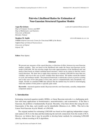
is known. We consider the situation where E(y do(x)) is reduced to anexpression without any do(·) operators.In the simplest case, the relation of x and y is acyclic, i.e., there is nodirected cycle in the causal structure, and the exogenous variables are independent, which implies that there are no latent confounders:x exy fy (x, ey ),(20)(21)where exogenous variables ex and ey are independent, in contrast to theSEM in Eq. (2)-(3). If some latent confounders do exist, this means theexogenous variables are dependent. The causal structure of the model isshown on the left of Fig. 2. In this case, it can straightforwardly be shownthat E(y do(x)) E(y x) (Pearl, 1995). Following this, the average causaleffect is calculated by the difference between two conditional expectations:E(y do(x d)) E(y do(x c)) E(y x d) E(y x c).(22)We can also describe a more general case, where the additional variableszq (q 1, · · · , Q) exist. Assume that the causal relations of x, y and zq(q 1, · · · , Q) are acyclic, and their exogenous variables are independent. Itmust now be decided which of the variables zi should be observed and usedto identify E(y do(x)). A sufficient set of variables for this is that of theparents of x, i.e., the variables that have directed edges to x (Pearl, 1995).Then, the average causal effect can be estimated byE(y do(x d)) E(y do(x c)) Epa(x) [E(y x d, pa(x))] Epa(x) [E(y x c, pa(x))],(23)where pa(x) denotes the set of parents of x. If fy is linear, the average causaleffect can be simplified to the difference (d c) multiplied by the partialregression coefficient of x when y is regressed on x and its parents. Anexample of a causal structure is given on the right of Fig. 2, where observingz1 and z4 is sufficient. Further details regarding latent confounder cases canbe found in Shpitser and Pearl (2006, 2008). Once the causal structure isknown, in many cases it is possible to determine whether average causaleffects are identifiable, i.e., can be uniquely estimated from the observeddata.2.5Identifiability of causal structuresIn this subsection, we discuss the identifiability of causal structures, i.e.,under which model assumptions the causal structure of variables can be11

uniquely estimated based on the observed data. Model assumptions represent the background knowledge and hypotheses of the modeler and placeconstraints on the SEM. These assumptions can sometimes be tested to detect possible violations, although, as in any data analysis process, it wouldbe impossible to prove that they are true.2.5.1Basic setupWe first explain the basic setup for identifying causal structures (Pearl, 2000;Spirtes et al., 1993). We assume that the causal relations of the observedvariables are acyclic, i.e., there are no directed cycles or feedback loops in thecausal graph. Since the exogenous variables are independent, it is impliedthat there are no latent or unobserved confounding variables that causallyinfluence more than one variable. Although these assumptions may appearto be restrictive, it is possible to relax the two assumptions and develop moregeneral methods based on the information obtained from the basic setup.In this paper, the focus is on continuous variable cases. Although nospecific functional form is assumed for discrete-valued data, in most cases,linearity and Gaussianity are assumed for continuous-valued data (Spirteset al., 1993; Pearl, 2000). This assumption of linearity would, however, almostcertainly be violated when analyzing real-world data. Therefore, in theory,nonlinear approaches are probably more suitable for modeling the causalrelations of variables. However, it should be noted that, in practice, linearmethods can often provide better results when finding qualititative relationsincluding causal directions is necessary (Pe’er and Hacohen, 2011; Hurleyet al., 2012), since nonlinear methods usually require very large sample sizes.In the remainder of the paper, we mainly discuss linear methods, but alsorefer to their nonlinear extensions. In the following sections, we furthermoreshow that the assumption of Gaussianity actually limits the applicabilityof causality estimation methods, and that a significant advantage may beachieved by departing from this assumption.The basic model for continuous observed variables xi (i 1, · · · , d) istherefore formulated as follows: A causal ordering of the variables xi is denoted by k(i). With this ordering, the causal relations of the variables xi canbe graphically represented by a directed acyclic graph (DAG)1) , so that nolater variable determines, that is, has a directed path to, any earlier variablein the DAG. Further, we assume that the functional relations of the variablesare linear. Without loss of generality, the variables xi are assumed to havezero mean. We thus obtain a linear acyclic SEM with no latent confounders12

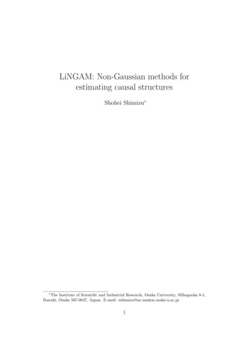
(Wright, 1921; Bollen, 1989):xi bij xj ei ,(24)k(j) k(i)where ei are continuous latent variables that are exogenous, i.e., are notdetermined inside the model, and bij are the connection strengths from xjto xi . The exogenous variables ei have zero mean and non-zero variance,and are independent of each other. The independence assumption betweenei implies that there are no latent confounding variables.In matrix form, the linear acyclic SEM with no latent confounders inEq. (24) can be written asx Bx e,(25)where the connection strength matrix B collects the connection strengths bij ,and the vectors x and e collect the observed variables xi and the exogenousvariables ei , respectively. The zero/non-zero pattern of bij corresponds tothe absence/existence pattern of the directed edges. That is, if bij ̸ 0,there is a directed edge from xj to xi , but if this is not the case, there is nodirected edge from xj to xi . Note that, due to the acyclicity, the diagonalelements of B are all zeros. It can be shown that it is always possible toperform simultaneous, equal row and column permutations on the connectionstrength matrix B to cause it to become strictly lower triangular, based onthe acyclicity assumption (Bollen, 1989). Here, strict lower triangularity isdefined as a lower triangular structure with the diagonal consisting entirelyof zeros.Examples of causal graphs for representing the linear acyclic SEMs withno latent confounders in Eq. (25) are provided in Fig. 3. The SEM corresponding to the left-most causal graph of the figure is written as e1x10 0 3x1 x2 5 0 0 x2 e2 .(26)e3x3x30 0 0In this example, x3 is in the first position of the causal ordering that causesB to be strictly lower triangular, x1 is in the second, and x2 is in the third,i.e., k(3) 1, k(1) 2, and k(2) 3. If we permute the variables x1 to x3according to the causal ordering, we obtain 0 0 0e3x3x3 x1 3 0 0 x1 e1 .(27)e2x2x20 5 013

It can be seen that the resulting connection strength matrix is strictly lowertriangular. There is no other such causal ordering of the variables that resultsin a strictly lower triangular structure in this example. In contrast, there aretwo such causal orderings in the center causal graph: i) k(1) 1, k(3) 2,and k(2) 3; and ii) k(3) 1, k(1) 2, and k(2) 3, since there is nodirected path between x1 and x3 .The goal of identifying causal structures under this basic setup is to estimate the unknown, B, by using only the data X, based on the assumption that X is randomly sampled from a linear acyclic SEM with no latentconfounders, as represented by Eq. (25) above. In other words, we aim todetermine which model is true among the class of linear acyclic SEMs withno latent confounders, assuming that the class includes the true one.2.5.2A conventional approachIn this section, we first discuss the identifiability problems experienced withconventional methods for estimating B of the linear acyclic SEM with nolatent confounders in Eq. (25). We say that B is identifiable if and onlyif B can be uniquely determined or estimated from the data distributionp(x). Once B is identified, we can estimate the causal structure from thezero/non-zero pattern of its elements, bij . The connection strength matrixB, together with the distribution of the exogenous variables p(e), induces thedistribution of the observed variables p(x). If p(x) are different for differentB, it follows that B can be uniquely determined.The causal Markov condition is a classical principle used for estimatingthe causal structure of the linear acyclic SEM with no latent confounders inEq. (25). For any linear acyclic SEM, the causal Markov condition holds2)(Pearl and Verma, 1991), as follows: Each observed variable xi is independentof its non-descendants in the DAG conditional on its parents, i.e., p(x) Πdi 1 p(xi pa(xi )). If Gaussianity of the exogenous variables is furthermoreassumed, conditional independence is reduced to partial uncorrelatedness.Thus, conditional independence between observed variables provides a clueas to what the underlying causal structure is.It is necessary to make an additional assumption, known as faithfulness(Spirtes et al., 1993) or stability (Pearl, 2000), when making use of the causalMarkov condition for estimating the causal structure. In this case, the faithfulness assumption means that the conditional independence of xi is represented by the graph structure only, i.e., by the zero/non-zero status of bij ,and not by the specific values of bij . Thus, owing to the faithfulness assumption, certain special cases are excluded, so that no conditional independenceof xi holds other than that derived from the causal Markov condition. The14

following is an example of faithfulness being violated:x exy x eyz x y ez ,(28)(29)(30)where ex , ey , ez are Gaussian and mutually independent. The associatedcausal graph is shown in Fig. 4. When the causal Markov condition is appliedto the causal graph

Non-Gaussian Acyclic Models (LiNGAM). We explain the basic LiNGAM model in Section 3, its estimation methods in Section 4 and its extensions in Section 5. Methods that form part of the LiNGAM group are capable of estimating a much wider variety of causal structures than classical methods. 2 Basics of causal inference