Transcription
8Copulas8.1 IntroductionCopulas are a popular method for modeling multivariate distributions. A copula models the dependence—and only the dependence—between the variatesin a multivariate distribution and can be combined with any set of univariatedistributions for the marginal distributions. Consequently, the use of copulasallows us to take advantage of the wide variety of univariate models that areavailable.A copula is a multivariate CDF whose univariate marginal distributionsare all Uniform(0,1). Suppose that Y (Y1 , . . . , Yd ) has a multivariate CDFFY with continuous marginal univariate CDFs FY1 , . . . , FYd . Then, by equation (A.9) in Section A.9.2, each of FY1 (Y1 ), . . . , FYd (Yd ) is Uniform(0,1) distributed. Therefore, the CDF of {FY1 (Y1 ), . . . , FYd (Yd )} is a copula. This CDFis called the copula of Y and denoted by CY . CY contains all informationabout dependencies among the components of Y but has no information aboutthe marginal CDFs of Y .It is easy to find a formula for CY . To avoid technical issues, in this sectionwe will assume that all random variables have continuous, strictly increasingCDFs. More precisely, the CDFs are assumed to be increasing on their support. For example, the exponential CDF½1 e y , y 0,F (y) 0,y 0,has support [0, ) and is strictly increasing on that set. The assumption thatthe CDF is continuous and strictly increasing is avoided in more mathematically advanced texts; see Section 8.8.Since CY is the CDF of {FY1 (Y1 ), . . . , FYd (Yd )}, by the definition of a CDFwe haveCY (u1 , . . . , ud ) P {FY1 (Y1 ) u1 , . . . , FYd (Yd ) ud }D. Ruppert, Statistics and Data Analysis for Financial Engineering, Springer Texts in Statistics,DOI 10.1007/978-1-4419-7787-8 8, Springer Science Business Media, LLC 2011175
1768 Copulas ª P Y1 FY 1(u1 ), . . . , Yd FY 1(ud )1d ª(u1 ), . . . , FY 1(ud ) . FY FY 11d(8.1)Next, letting uj FYj (yj ), j 1, . . . , d, in (8.1) we see thatFY (y1 , . . . , yd ) CY {FY1 (y1 ), . . . , FYd (yd )} .(8.2)Equation (8.2) is part of a famous theorem due to Sklar which states that theFY can be decomposed into the copula CY , which contains all informationabout the dependencies among (Y1 , . . . , Yd ), and the univariate marginal CDFsFY1 , . . . , FYd , which contain all information about the univariate marginaldistributions.Let dcY (u1 , . . . , ud ) CY (u1 , . . . , ud )(8.3) u1 · · · udbe the density of CY . By differentiating (8.2), we find that the density of Yis equal tofY (y1 , . . . , yd ) cY {FY1 (y1 ), . . . , FYd (yd )}fY1 (y1 ) · · · fYd (yd ).(8.4)One important property of copulas is that they are invariant to strictlyincreasing transformations of the variables. More precisely, suppose that gj isstrictly increasing and Xj gj (Yj ) for j 1, . . . , d. Then X (X1 , . . . , Xd )and Y have the same copulas. To see this, first note that the CDF of X isFX (x1 , . . . , xd ) P {g1 (Y1 ) x1 , . . . , gd (Yd ) xd }ª P Y1 g1 1 (x1 ), . . . , Yd gd 1 (xd ) ª FY g1 1 (x1 ), . . . , gd 1 (xd )(8.5)and therefore the CDF of Xj is ªFXj (xj ) FYj gj 1 (xj ) .Consequently,no 1 1FFX(u) g(u)jYjj(8.6)and by (8.1) applied to X, (8.5), (8.6), and then (8.1) applied to Y , the copulaof X is 1ª 1CX (u1 , . . . , ud ) FX FX(u1 ), . . . , FX(ud )1d 1 1ªª (u1 ) , . . . , gd 1 FX(ud ) FY g1 1 FX1d ª(u1 ), . . . , FY 1(ud ) FY FY 11d CY (u1 , . . . , ud ).To use copulas to model multivariate dependencies, we need parametricfamilies of copulas. We turn to that topic next.
8.3 Gaussian and t-Copulas1778.2 Special CopulasThere are three copulas of special interest because they represent independence and the two extremes of dependence.The d-dimensional independence copula is the copula of d independentuniform(0,1) random variables. It equalsC ind (u1 , . . . , ud ) u1 · · · ud ,(8.7)and has a density that is uniform on [0, 1]d , that is, its density is c ind (u1 , . . . ,ud ) 1 on [0, 1]d .The d-dimensional co-monotonicity copula C M has perfect positive dependence. Let U be Uniform(0,1). Then, the co-monotonicity copula is theCDF of U (U, . . . , U ); that is, U contains d copies of U so that all of thecomponents of U are equal. Thus,C M (u1 , . . . , ud ) P (U u1 , . . . , U ud ) P {Y min(u1 , . . . , ud )} min(u1 , . . . , ud ).The two-dimensional counter-monotonicity copula C CM copula is the CDFof (U, 1 U ), which has perfect negative dependence. Therefore,C CM (u1 , u2 ) P (U u1 & 1 U u2 ) P (1 u2 U u1 ) max(u1 u2 1, 0).(8.8)It is easy to derive the last equality in (8.8). If 1 u2 u1 , then the event{1 u2 U u1 } is impossible so the probability is 0. Otherwise, theprobability is the length of the interval (1 u2 , u1 ), which is u1 u2 1.It is not possible to have a counter-monotonicity copula with d 2. If, forexample, U1 is counter-monotonic to U2 and U2 is counter-monotonic to U3 ,then U1 and U3 will be co-monotonic, not counter-monotonic.8.3 Gaussian and t-CopulasMultivariate normal and t-distributions offer a convenient way to generatefamilies of copulas. Let Y (Y1 , . . . , Yd ) have a multivariate normal distribution. Since CY depends only on the dependencies within Y , not the univariate marginal distributions, CY depends only on the correlation matrix of Y ,which will be denoted by Ω. Therefore, there is a one-to-one correspondencebetween correlation matrices and Gaussian copulas. The Gaussian copula withcorrelation matrix Ω will be denoted C Gauss ( · Ω).If a random vector Y has a Gaussian copula, then Y is said to havea meta-Gaussian distribution. This does not, of course, mean that Y has amultivariate Gaussian distribution, since the univariate marginal distributionsof Y could be any distributions at all. A d-dimensional Gaussian copula whose
1788 Copulascorrelation matrix is the identity matrix, so that all correlations are zero, is thed-dimensional independence copula. A Gaussian copula will converge to theco-monotonicity copula if all correlations in Ω converge to 1. In the bivariatecase, as the correlation converges to 1, the copula converges to the countermonotonicity copula.Similarly, let C t ( · ν, Ω) be the copula of a multivariate t-distributionwith correlation matrix Ω and degrees of freedom ν.1 The shape parameterν affects both the univariate marginal distributions and the copula, so ν isa parameter of the copula. We will see in Section 8.6 that ν determines theamount of tail dependence in a t-copula. A distribution with a t-copula iscalled a t-meta distribution.8.4 Archimedean CopulasAn Archimedean copula with a strict generator has the formC(u1 , . . . , ud ) φ 1 {φ(u1 ) · · · φ(ud )},(8.9)where the function φ is the generator of the copula and satisfies1. φ is a continuous, strictly decreasing, and convex function mapping [0, 1]onto [0, ],2. φ(0) , and3. φ(1) 0.Figure 8.1 is a plot of a generator and illustrates these properties. It ispossible to relax assumption 2, but then the generator is not called strictand construction of the copula is more complex. There are many families ofArchimedean copulas, but we will only look at three, the Clayton, Frank, andGumbel copulas.Notice that in (8.9), the value of C(u1 , . . . , ud ) is unchanged if we permuteu1 , . . . , ud . A distribution with this property is called exchangeable. One consequence of exchangeability is that both Kendall’s and Spearman’s rank correlation introduced later in Section 8.5 are the same for all pairs of variables.Archimedean copulas are most useful in the bivariate case or in applicationswhere we expect all pairs to have similar dependencies.8.4.1 Frank CopulaThe Frank copula has generator½ θu¾e 1,φFr (u) loge θ 11 θ .There is a minor technical issue here if ν 2. In this case, the t-distribution doesnot have covariance and correlation matrices. However, it still has a scale matrixand we will assume that the scale matrix is equal to some correlation matrix Ω.
1796024φ(u)810128.4 Archimedean Copulas0.00.20.40.60.81.0uFig. 8.1. Generator of the Frank copula with θ 1.The inverse generator is(φFr ) 1 (y) log e y {e θ 1} 1.θTherefore, by (8.9), the bivariate Frank copula is½¾(e θu1 1)(e θu2 1)1FrC (u1 , u2 ) log 1 .θe θ 1(8.10)The case θ 0 requires some care, since plugging this value into (8.10) gives0/0. Instead, one must evaluate the limit of (8.10) as θ 0. Using the approximations ex 1 x and log(1 x) x as x 0, one can show that asθ 0, C Fr (u1 , u2 ) u1 u2 , the bivariate independence copula. Therefore, forθ 0 we define the Frank copula to be the independence copula.It is interesting to study the limits of C Fr (u1 , u2 ) as θ . As θ ,the bivariate Frank copula converges to the counter-monotonicity copula. Tosee this, first note that as θ ,on1(8.11)C Fr (u1 , u2 ) log 1 e θ(u1 u2 1) .θIf u1 u2 1 0, then as θ , the exponent θ(u1 u2 1) in (8.11)converges to and
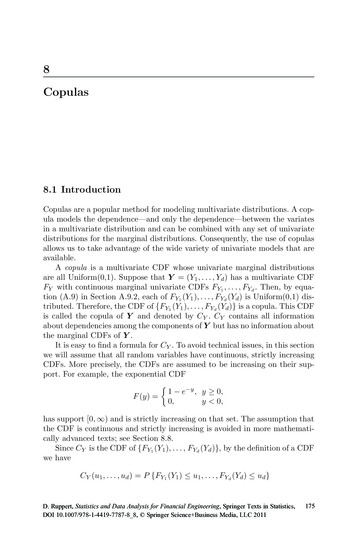
8 Copulas0.80.00.40.80.0θ 0θ 5u20.0u20.00.40.80.00.40.80.00.4u1u1θ 20θ 50θ 500u20.00.8u10.80.0u20.6u10.40.80.6θ u2θ 100.6u20.6θ 500.0u2θ 1000.61800.00.40.80.0u10.40.8u1Fig. 8.2. Random samples from Frank copulas.onlog 1 e θ(u1 u2 1) θ(u1 u2 1)so that C Fr (u1 , u2 ) u1 u2 1. If u1 u2 1 0, then θ(u1 u2 1) and C Fr (u1 , u2 ) 0. Putting these results together, we see that C Fr (u1 , u2 )converges to max(0, u1 u2 1), the counter-monotonicity copula, as θ .As θ , C Fr (u1 , u2 ) min(u1 , u2 ), the co-monotonicity copula. Verification of this is left as an exercise for the reader.Figure 8.2 contains scatterplots of bivariate samples from nine Frank copulas, all with a sample size of 200 and with values of θ that give dependenciesranging from strongly negative to strongly positive. The convergence to thecounter-monotonicity (co-monotonicity) copula as θ ( ) can be seenin the scatterplots.8.4.2 Clayton CopulaThe Clayton copula, with generator (t θ 1)/θ, θ 0, is
8.4 Archimedean Copulas181 θ 1/θC Cl (u1 , . . . , ud ) (u θ.1 · · · ud d 1)We define the Clayton copula for θ 0 as the limitlim C Cl (u1 , . . . , ud ) u1 · · · udθ 0which is the independence copula. There is another way to derive this result.As θ 0, l’Hôpital’s rule shows that the generator (t θ 1)/θ converges toφ(t) log(t) with inverse φ 1 (t) exp( t). Therefore,C Cl (u1 , . . . , ud ) φ 1 {φ(u1 ) · · · φ(ud )} exp { ( log u1 · · · log ud )} u1 · · · ud .It is possible to extend the range of θ to include 1 θ 0, but then thegenerator (t θ 1)/θ is finite at t 0 in violation of assumption 2. of strictgenerators. Thus, the generator is not strict if θ 0. As a result, it is necessaryto define C Cl (u1 , . . . , ud ) to equal 0 for small values of ui . To appreciate this, θconsider the bivariate case. If 1 θ 0, then u θ1 u2 1 0 occursClwhen u1 and u2 are both small. In these cases, C (u1 , u2 ) is set equal to 0. θTherefore, there is no probability in the region u θ1 u2 1 0. In the limit,as θ 1, there is no probability in the region u1 u2 1.As θ 1, the bivariate Clayton copula converges to the countermonotonicity copula, and as θ , the Clayton copula converges to theco-monotonicity copula.Figure 8.3 contains scatterplots of bivariate samples from Clayton copulas,all with a sample size of 200 and with values of θ that give dependenciesranging from counter-monotonicity to co-monotonicity. Comparing Figures8.2 and 8.3, we see that the Frank and Clayton copulas are rather differentwhen the amount of dependence is somewhere between these two extremes. θIn particular, the Clayton copula’s exclusion of the region u θ1 u2 1 0when θ 0 is evident, especially in the example with θ 0.7. In contrast,the Frank copula has positive probability on the entire unit square. The Frankcopula is symmetric about the diagonal from (0, 1) to (1, 0), but the Claytoncopula does not have this symmetry.8.4.3 Gumbel CopulaThe Gumbel copula has generator { log(t)}θ , θ 1, and consequently isequal toh ª1/θ i.C Gu (u1 , . . . , ud ) exp (log u1 )θ · · · (log ud )θThe Gumbel copula is the independence copula when θ 1 and converges tothe co-monotonicity copula as θ , but the Gumbel copula cannot havenegative dependence.
8 Copulasu20.00.40.80.0θ 0.1θ 0.1θ 10.8u20.00.40.8u20.40.00.40.00.40.80.00.4u1u1θ 5θ 15θ 00.40.80.0u2θ 0.30.8θ 0.70.8θ 0.980.41820.00.4u10.80.00.40.8u1Fig. 8.3. Random samples of size 200 from Clayton copulas.Figure 8.4 contains scatterplots of bivariate samples from Gumbel copulas,with a sample size of 200 and with values of θ that give dependencies rangingfrom near independence to strong positive dependence.In applications, it is useful that the different copula families have differentproperties, since this increases the likelihood of finding a copula that fits thedata.8.5 Rank CorrelationThe Pearson correlation coefficient defined by (4.3) is not convenient for fittingcopulas to data, since it depends on the univariate marginal distributions aswell as the copula. Rank correlation coefficients remedy this problem, sincethey depend only on the copula.For each variable, the ranks of that variable are determined by orderingthe observations from smallest to largest and giving the smallest rank 1, thenext-smallest rank 2, and so forth. In other words, if Y1 , . . . , Yn is a sample,
8.5 Rank Correlationθ 1.50.8u20.00.00.40.80.00.4u1u1u1θ 4θ 8θ 8u20.00.40.80.0u2θ 20.40.40.0u20.8θ 1.11830.0u10.40.80.00.4u10.8u1Fig. 8.4. Random samples from Gumbel copulas.then the rank of Yi in the sample is equal to 1 if Yi is the smallest observation,is 2 if Y2 is the second smallest, and so forth. More mathematically, the rankof Yi can be defined also by the formularank(Yi ) nXI(Yj Yi ),(8.12)j 1which counts the number of observations (including Yi itself) that are lessthan or equal to Yi . A rank statistic is a statistic that depends on the dataonly through the ranks. A key property of ranks is that they are unchanged bystrictly monotonic transformations. In particular, the ranks are unchanged bytransforming each variable by its CDF, so the distribution of any rank statisticdepends only on the copula of the data, not on the univariate marginals.We will be concerned with rank statistics that measure statistical association between pairs of variables. These statistics are called rank correlations.There are two rank correlation coefficients in widespread usage, Kendall’s tauand Spearman’s rho.8.5.1 Kendall’s TauLet (Y1 , Y2 ) be a bivariate random vector and let (Y1 , Y2 ) be an independentcopy of (Y1 , Y2 ). Then (Y1 , Y2 ) and (Y1 , Y2 ) are called a concordant pair if
1848 Copulasthe ranking of Y1 relative to Y1 is the same as the ranking of Y2 relative toY2 , that is, either Y1 Y1 and Y2 Y2 or Y1 Y1 and Y2 Y2 . In eithercase, (Y1 Y1 )(Y2 Y2 ) 0. Similarly, (Y1 , Y2 ) and (Y1 , Y2 ) are called adiscordant pair if (Y1 Y1 )(Y2 Y2 ) 0. Kendall’s tau is the probabilityof a concordant pair minus the probability of a discordant pair. Therefore,Kendall’s tau for (Y1 , Y2 ) isρτ (Y1 , Y2 ) P {(Y1 Y1 )(Y2 Y2 ) 0} P {(Y1 Y1 )(Y2 Y2 ) 0}(8.13) E [sign{(Y1 Y1 )(Y2 Y2 )}] ,where the sign function is(sign(x) 1, 1,0,x 0,x 0,x 0.It is easy to check that if g and h are increasing functions, thenρτ {g(Y1 ), h(Y2 )} ρτ (Y1 , Y2 ).(8.14)Stated differently, Kendall’s tau is invariant to monotonically increasing transformations. If g and h are the marginal CDFs of Y1 and Y2 , then the left-handside of (8.14) is the value of Kendall’s tau for the copula of (Y1 , Y2 ). This showsthat Kendall’s tau depends only on the copula of a bivariate random vector.For a random vector Y , we define the Kendall tau correlation matrix to bethe matrix whose (j, k) entry is Kendall’s tau for the jth and kth componentsof Y .If we have a bivariate sample Y i (Yi,1 , Yi,2 ), i 1, . . . , n, then thesample Kendall’s tau isµ ¶ 1nρbτ (Y1 , Y2 ) 2Xsign {(Yi,1 Yj,1 )(Yi,2 Yj,2 )} .(8.15)1 i j nµ ¶nis the number of summands in (8.15), so ρb is sign{(Yi,1 Yj,1 )2(Yi,2 Yj,2 )} averaged across all distinct pairs and is a sample version of (8.13).Note that8.5.2 Spearman’s Correlation CoefficientFor a sample, Spearman’s correlation coefficient is simply the usual Pearsoncorrelation calculated from the ranks of the data. For a distribution (that is,an infinite population rather than a finite sample), both variables are transformed by their CDFs and then the Pearson correlation is computed from thetransformed variables. Transforming a random variable by its CDF is analogous to computing the ranks of a variable in a finite sample.
8.6 Tail Dependence185Stated differently, Spearman’s correlation coefficient, also called Spearman’s rho, for a bivariate random vector (Y1 , Y2 ) will be denoted by ρS (Y1 , Y2 )and is defined to be the Pearson correlation coefficient of {FY1 (Y1 ), FY2 (Y2 )}:ρS (Y1 , Y2 ) Corr{FY1 (Y1 ), FY2 (Y2 )}.Since the distribution of {FY1 (Y1 ), FY2 (Y2 )} is the copula of (Y1 , Y2 ), Spearman’s rho, like Kendall’s tau, depends only on the copula.The sample version of Spearman’s correlation coefficient can be computedfrom the ranks of the data and for a bivariate sample Y i (Yi,1 , Yi,2 ), i 1, . . . , n, is¾½¾n ½X12n 1n 1) ) rank(Yrank(Y.i,1i,2n(n2 1) i 122(8.16)The set of ranks for any variable is, of course, the integers 1 to n and (n 1)/2is the mean of its ranks. It can be shown that ρbS (Y1 , Y2 ) is the sample Pearsoncorrelation between the ranks of Yi,1 and the ranks of Yi,2 .2If Y (Y1 , . . . , Yd ) is a random vector, then the Spearman correlationmatrix of Y is the correlation matrix of {FY1 (Y1 ), . . . , FYd (Yd )} and containsthe Spearman correlation coefficients for all pairs of coordinates of Y . Thesample Spearman correlation matrix is defined analogously.ρbS (Y1 , Y2 ) 8.6 Tail DependenceTail dependence measures association between the extreme values of two random variables and depends only on their copula. We will start with lower taildependence, which uses extremes in the lower tail. Suppose that Y (Y1 , Y2 )is a bivariate random vector with copula CY . Then the coefficient of lowertail dependence is denoted by λl and defined as ª(q) Y1 FY 1(q)(8.17)λl : lim P Y2 FY 121q 0 ªP Y2 FY 1(q) and Y1 FY 1(q)21 ª lim(8.18)q 0P Y1 FY 1(q)1P {FY2 (Y2 ) q and FY1 (Y1 ) q}q 0P {FY1 (Y1 ) q}CY (q, q). limq 0q lim2(8.19)(8.20)If there are ties, then ranks are averaged among tied observations. For example,if there are two observations tied for smallest, then they each get a rank of 1.5.When there are ties, then these results must be modified.
1868 CopulasIt is helpful to look at these equations individually. As elsewhere in this chapter, for simplicity we are assuming that FY1 and FY2 are strictly increasing ontheir supports and therefore have inverses.First, (8.17) defines λl as the limit as q 0 of the conditional probabilitythat Y2 is less than or equal to its qth quantile, given that Y1 is less than orequal to its qth quantile. Since we are taking a limit as q 0, we are lookingat the extreme left tail. What happens if Y1 and Y2 are independent? ThenP (Y2 y2 Y1 y1 ) P (Y2 y2 ) for all y1 and y2 . Therefore, the conditional(q)) andprobability in (8.17) equals the unconditional probability P (Y2 FY 12this probability converges to 0 as q 0. Therefore, λl 0 implies that in theextreme left tail, Y1 and Y2 behave as if they were independent.Equation (8.18) is just the definition of conditional probability. Equation(8.19) is simply (8.18) after applying the probability transformation to bothvariables.The numerator in equation (8.20) is just the definition of a copula andthe denominator is the result of FY1 (Y1 ) being Uniform(0,1) distributed; see(A.9).Deriving formulas for λl for Gaussian and t-copulas is a topic best leftfor more advanced books. Here we give only the results; see Section 8.8 forfurther reading. For any Gaussian copula with ρ 6 1, λl 0, that is, Gaussiancopulasdo not have tail dependence except in the extreme case of perfectpositive correlation. For a t-copula with ν degrees of freedom and correlationρ,)( sλl 2Ft,ν 1 (ν 1)(1 ρ)1 ρ,(8.21)where Ft,ν 1 is the CDF of the t-distribution with ν 1 degrees of freedom.Since Ft,ν 1 ( ) 0, we see that λl 0 as ν , which makes sensesince the t-copula converges to a Gaussian copula as ν . Also, λl 0as ρ 1, which is also not too surprising, since ρ 1 is perfect negativedependence and λl measures positive tail dependence.The coefficient of upper tail dependence, λu , is ª(q) Y1 FY 1(q)(8.22)λu : lim P Y2 FY 121q 1 2 limq 11 CY (q, q).1 q(8.23)We see that λu is defined analogously to λl ; λu is the limit as q 1 of theconditional probability that Y2 is greater than or equal to its qth quantile,given that Y1 is greater than or equal to its qth quantile. Deriving (8.23) isleft as an exercise for the interested reader.For Gaussian and t-copula, λu λl , so that λu 0 for any Gaussian copula and for a t-copula, λl is given by the right-hand side of (8.21). Coefficientsof tail dependence for t-copulas are plotted in Figure 8.5. One can see λl λudepends strongly on both ρ and ν.
1.08.7 Calibrating Copulas0.40.60.8ν 1ν 4ν 25ν 2500.00.2λl λu187 1.0 0.50.00.51.0ρFig. 8.5. t-copulas coefficients of tail dependence as functions of ρ for ν 1, 4, 25,and 250.For the independence copula, λl and λu are both equal to 0, and for theco-monotonicity copula both are equal to 1.Knowing whether or not there is tail dependence is important for riskmanagement. If there are no tail dependencies among the returns on the assetsin a portfolio, then there is little risk of clusters of very negative returns, andthe risk of an extreme negative return on the portfolio is low. Conversely, ifthere are tail dependencies, then the likelihood of extreme negative returnsoccurring simultaneously on several assets in the portfolio can be high.8.7 Calibrating CopulasAssume that we have an i.i.d. sample Y i (Yi,1 , . . . , Yi,d ), i 1, . . . , n, andwe wish to estimate the copula of Y i and perhaps its marginal distributionsas well.An important task is choosing a copula model. The various copula modelsdiffer notably from each other. For example, some have tail dependence andothers do not. The Gumbel copula allows only positive dependence or independence. The Clayton copula with negative dependence excludes the regionwhere both u1 and u2 are small. As will be seen in this section, an appropriatecopula model can be selected using graphical techniques as well as with AIC.
1888 Copulas8.7.1 Maximum LikelihoodSuppose we have parametric models FY1 (· θ 1 ), . . . , FYd (· θ d ) for the marginalCDFs as well as a parametric model cY (· θ C ) for the copula density. By takinglogs of (8.4), we find that the log-likelihood is÷ nn o X L(θ 1 , . . . , θ d , θ C ) log cY FY1 (Yi,1 θ 1 ), . . . , FYd (Yi,d θ d ) θ Ci 1! ª ª log fY1 (Yi,1 θ 1 ) · · · log fYd (Yi,d θ d ) . (8.24)Maximum likelihood estimation finds the maximum of L(θ 1 , . . . , θ d , θ C ) overthe entire set of parameters (θ 1 , . . . , θ d , θ C ).There are two potential problems with maximum likelihood estimation.First, because of the large number of parameters, especially for large values ofd, maximizing L(θ 1 , . . . , θ d , θ C ) can be a challenging numerical problem. Thisdifficulty can be ameliorated by the use of starting values that are close to theMLEs. The pseudo-maximum likelihood estimates discussed in the next section are easier to compute than the MLE and can used either as an alternativeto the MLE or as starting values for the MLE.Second, maximum likelihood estimation requires parametric models forboth the copula and the marginal distributions. If any of the marginal distributions are not well fit by a convenient parametric family, this may causebiases in the estimated parameters of both the marginal distributions andthe copula. The semiparametric approach to pseudo-maximum likelihood estimation, where the marginal distributions are estimated nonparametrically,provides a remedy to this problem.8.7.2 Pseudo-Maximum LikelihoodPseudo-maximum likelihood estimation is a two-step process. In the first step,each of the d marginal distribution functions is estimated, one at a time. LetFbYj be the estimate of the jth marginal CDF, j 1, . . . , d. In the second step,nX· n o log cY FbY1 (Yi,1 ), . . . , FbYd (Yi,d ) θ C(8.25)i 1is maximized over θ C . Note that (8.25) is obtained from (8.24) by deletingterms that do not depend on θ C and replacing the marginal CDFs by estimates. By estimating parameters in the marginal distributions and in thecopula separately, the pseudo-maximum likelihood approach avoids a highdimensional optimization.There are two approaches to step 1, parametric and nonparametric. Inthe parametric approach, parametric models FY1 (· θ 1 ), . . . , FYd (· θ d ) for the
8.7 Calibrating Copulas189marginal CDFs are assumed as in maximum likelihood estimation. The dataY1,j , . . . , Yn,j for the jth variate are used to estimate θ j , usually by maximumbj ). In the nonlikelihood as discussed in Chapter 5. Then, FbYj (·) FYj (· θbparametric approach, FYj is estimated by the empirical CDF of Y1,j , . . . , Yn,j ,except that the divisor n in (4.1) is replaced by n 1 so thatPnI{Yi,j y}b.(8.26)FYj (y) i 1n 1With this modified divisor, the maximum value of FbYj (Yi,j ) is n/(n 1)rather than 1. Avoiding a value of 1 is essential when, as is often the case,cY (u1 , . . . , ud θ C ) if some of u1 , . . . , ud are equal to 1.When both steps are parametric, the estimation method is called parametric pseudo-maximum likelihood. The combination of a nonparametric step 1and a parametric step 2 is called semiparametric pseudo-maximum likelihood.In the second step of pseudo-maximum likelihood, the maximization canbe difficult when θ C is high-dimensional. For example, if one uses a Gaussianor t-copula, then there are d(d 1)/2 correlation parameters. One way tosolve this problem is to assume some structure to the correlation. An extremecase of this is the equi-correlation model where all nondiagonal elements ofthe correlation matrix have a common value, call it ρ. If one is reluctant toassume some type of structured correlation matrix, then it is essential to havegood starting values for the correlation matrix when maximizing (8.25). ForGaussian and t-copulas, starting values can be obtained via rank correlationsas discussed in the next section.The values FbYj (Yi,j ), i 1, . . . , n and j 1, . . . , d, will be called theuniform-transformed variables, since they should have approximately Uniform(0,1) distributions. The multivariate empirical CDF [see equation (A.38)]of the uniform-transformed variables is called the empirical copula and is anonparametric estimate of the copula. The empirical copula is useful for checking the goodness of fits of parametric copula models; see Example 8.2.8.7.3 Calibrating Meta-Gaussian and Meta-t-DistributionsGaussian CopulasRank correlation can be useful for estimating the parameters of a copula.Suppose Y i (Yi,1 , . . . , Yi,d ), i 1, . . . , n, is an i.i.d. sample from a metaGaussian distribution. Then its copula is C Gauss ( · Ω) for some correlationmatrix Ω. To estimate the distribution of Y , we need to estimate the univariate marginal distributions and Ω. The marginal distribution can be estimatedby the methods discussed in Chapter 5. Result (8.28) in the following theoremshows that Ω can be estimated by the sample Spearman correlation matrix.Theorem 8.1. Let Y (Y1 , . . . , Yd ) have a meta-Gaussian distribution withcontinuous marginal distributions and copula C Gauss ( · Ω) and let Ωi,j be thei, jth entry of Ω. Then
1908 Copulas2arcsin(Ωi,j ), andπ6ρS (Yi , Yj ) arcsin(Ωi,j /2) Ωi,j .πρτ (Yi , Yj ) (8.27)(8.28)Suppose, instead, that Y i , i 1, . . . , n, has a meta t-distribution withcontinuous marginal distributions and copula C t ( · ν, Ω). Then (8.27) stillholds, but (8.28) does not hold.The approximation in (8.28) uses the result that6arcsin(x/2) x for x 1.π(8.29)The left- and right-hand sides of (8.29) are equal when x 1, 0, 1 and theirmaximumdifference overªthe range 1 x 1 is 0.018. However, the relative error π6 arcsin(x/2) x / π6 arcsin(x/2) can be larger, as much as 0.047, andis largest near x 0.By (8.28), the sample Spearman rank correlation matrix Y i , i 1, . . . , n,can be used as an estimate of the correlation matrix Ω of C Gauss ( · Ω). Thisestimate could be the final one or could be used as a starting value for maximum likelihood or pseudo-maximum likelihood estimation.t-CopulasIf {Y i (Yi,1 , . . . , Yi,d ), i 1, . . . , n} is a sample from a distribution with at-copula, C t ( · ν, Ω), then we can use (8.27) and the sample Kendall’s taus toestimate Ω. Let ρbτ (Yj , Yk ) be the sample Kendall’s tau calculated using thesamples {Y1,j , . . . , Yn,j } and {Y1,k , . . . , Yn,k } of the jth and kth variables, ande wille be the matrix whose j, kth entry is sin{ π ρbτ (Yj , Yk )}. Then Ωlet Ω2have two of the three properties of a correlation matrix; it will be symmetricwith all diagonal entries equal to 1. However, it may not be positive definite,or even semidefinite, because some of its eigenvalues may be negative.e to estimate Ω.If all its eigenvalues are positive, then we will use Ω e slightly to make it positive definite. By (A.47),Otherwise, we alter Ωe O diag(λi ) O TΩe whe
between correlation matrices and Gaussian copulas. The Gaussian copula with correlation matrix › will be denoted CGauss( j›). If a random vector Y has a Gaussian copula, then Y is said to have a meta-Gaussian distribution. This does not, of course, mean that Y has a multivariate