WIXLIB

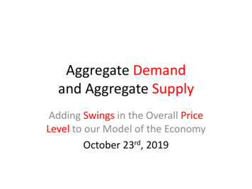
Aggregate Demandand Aggregate SupplyAdding Swings in the Overall PriceLevel to our Model of the EconomyOctober 23rd, 2019

AS/AD Model: Links output changesto changes in the price level Powell driving the bus. Targeting output andprices. AE model looks only at output swings. How do changes in demand affect aggregateoutput and the price level? How do changes in supply affect aggregateoutput and the price level? How do changes in the price level affectaggregate demand and aggregate output?

A Downward Sloping AD Curve:(As the overall price level falls, the level of output rises)

Is it due to the Substitution Effect?Demand curves, for specific goods,are downward sloping: As we travel down a demand curve wediscover:the quantity demanded rises, as the price fallsASSUMING ALL OTHER PRICES ARE STABLE! When the price of the good falls people buymore,Because the good is now CHEAPER THAN OTHER GOODS

A micro example, demand curvesworking, for an individual market. Microeconomic theory teaches us:When the price of an individual good falls,demand rises (the law of demand). If the price of solar power falls, and the price ofoil and coal stay the same, the demand for solarpower will rise. We substitute solar power for coal power, due tothe fall in the price of solar power.

The AD Curve: Substitution Effects CannotExplain the Downward slope of the AD Curve The Aggregate Demand Curve depicts theeffects on OVERALL DEMAND, given a changein the PRICES OF ALL GOODS AND SERVICES. Clearly substitution of one good for anothercannot explain a shift in overall demand givena shift in overall prices.

Why Does the Aggregate Demand Curve Slope Downward?(Why Is a Fall in the Overall Price Level,Associated with Higher Output?) The Wealth Effect:“Household consumption is most strongly determine by income, but it isalso affected by wealth.Some household wealth is held in nominal assets; so as price levels rise, thereal value of household wealth declines. This results in less consumption.” The Interest Rate Effect: “When prices rise, households and firms need more money tofinance buying and selling. This increase in demand for money causes the “price” ofholding money (the interest rate) to rise, discouraging firminvestment.”

The Wealth Effect: Ernie has SAVED 20,000, held in a local bank. A moped cost 8,900. A 12 foot flat screen TVcosts 9,200. A vacation to Paris for a monthcost 9,700. He contemplates buying two ofthese three items, after graduation. Prices, however, leap(inflation is 20%, in2018). New prices:Moped 10,680 TV 11,040 Vaca. 11,640 Ernie now can buy only one of the items.

The Interest Rate Effect(theoretical) Households keep their financial wealth invarious places: cash, bonds, stocks Households hold enough cash to make it easyto pay their bills If prices jump, households must sell somebonds and stocks to increase their cashholdings Sell bonds, prices fall, interest rates rise Higher interest rates means less investment

The Interest Rate Effect Explained(A Sesame Street Example) Bert, Ernie, Big Bird, Miss Piggy and the Count allkeep , on average, 5,000 in their checkingaccount, to pay bills. Prices fall(inflation is -1% in 2015) They each decide they only need 3,000 in theiraccounts now, to pay bills. They all buy bonds, the prices rise, and yields fall. The lower real interest rates boosts homebuilding.

A movement along the AD Curve:the price level falls and output rises

A shift in the AD Curve:

AE Model to AD-AS Modela simple derivation Our AE model assumes the overall price level is fixed.this reflects our assumption that there is enoughcapacity to increase output We relax that assumption. Prices jump from period 1 to period 2 The AE line falls, at any level of output less indemanded. Equilibrium is now lower. Thus we can ‘derive’ the AD line, by manipulating ourAE model

The AE Model: ‘Embedded’ in the AD-AS ModelSuppose inflation jumps. The price level rises to 110, from 100.Wealth effect and interest rate effect push down AE, for a given level of Y (AE1 falls to AE2)at P 100, equilibrium level for Y Y1at P 110, equilibrium level for Y Y2, lower than Y1

Shifts of the AD curve, vs. movements along itThe AD curve: relationshipbetween the price level andreal GDP demanded, holdingeverything else constant.A change in the price level notcaused by a component of realGDP changing results in amovement along the AD curve.A change in some componentof aggregate demand, on theother hand, will shift the ADcurve. 2013 Pearson Education, Inc. Publishing as Prentice Hall15 of 47

AD shifts: changes in fiscal policyBudget policy: The White House and the Congress can choose toincrease spending or cut taxes, as they did late in 2017. Other thingsequal, this will raise demand as it shifts the AD curve outward.In contrast, Senate Majority Leader Mitch McConnell’s recent calls tocut social security and Medicare payments, other things equal, wouldcause the AD curve to shift inward.shifts the aggregateA decrease in spendingdemand curve inward 2013 Pearson Education, Inc. Publishing as Prentice HallTable 13.116 of 47

AD shifts: changes in monetary policyMonetary policy: Chair Powell at the Federal Reserve can choose tochange interest rates, (think Phillips Curve) to pursue macroeconomicpolicy objectives.If the Federal Reserve lifts interest rates, investment spending falls;if the Fed lowers interest rates, investment spending rises.An increase in 2013 Pearson Education, Inc. Publishing as Prentice Hallshifts the aggregatedemand curve Table 13.1because 17 of 47

AD shifts: changes in expectationsTrump promises a business friendly environment: Households or firmsbecome more optimistic about the future, increasing consumption orinvestment respectively.N. Korea bombs Guam, The opposite would clearly occur.An increase in 2013 Pearson Education, Inc. Publishing as Prentice Hallshifts the aggregatedemand curve Table 13.1because 18 of 47

AD shifts: think 2015 Developing World vs. USABrazil and many emerging economies, in 2015, fell into recessions. Theirincomes and spending shrunk. Their imports of U.S. goods fell.Brazil’s exchange rate fell sharply. U.S. exports became more expensive,so foreigners bought less of them (and we bought more imports, also).An increase in 2013 Pearson Education, Inc. Publishing as Prentice Hallshifts the aggregatedemand curve Table 13.1because 19 of 47

The change in the U.S. real net exports in 2016-2019Q2:Subtracted 0.5% from real GDP

Aggregate supply and time frameAggregate supply refers to the quantity of goods and services that firmsare willing and able to supply.The relationship between this quantity and the price level is different inthe long and short run.So we will develop both a short-run and long-run aggregate supplycurve.Long-run aggregate supply curve: A curve that shows the relationship inthe long run between the price level and the quantity of real GDPsupplied. 2013 Pearson Education, Inc. Publishing as Prentice Hall21 of 47

Long-run aggregate supply curveIn the long run, the level of real GDP is determined by the number ofworkers, the level of technology, and the capital stock (factories,machinery, etc.).None of these elements are affected by the price level.So the long-runaggregate supply curvedoes not depend onthe price level; it is avertical line, at thelevel of potential orfull-employment GDP. 2013 Pearson Education, Inc. Publishing as Prentice HallFigure 13.222 of 47

The vertical long run supply curve: You can’tget more output if you allow more inflationThe same concept as the Phillips Curve:there is no LONG RUN inflation/unemployment tradeoff In the short run, there is evidence that aneconomy can produce more stuff, if you ignore arising price level. Chair Powell, driving the bus, could say,‘to hell with high inflation, I’ll accept it to getstronger growth and lower unemployment.’But the LONG TERM trajectory for output cannot belifted by allowing prices to rise faster.As we learned:LTSG %Δ in Labor Productivity %Δ in Labor Force

The Short run Aggregate Supply Curve:Why is it Upward Sloping? Who provides us with the output(the supply)?FIRMS What drives firm decisions?PROFITS The Simplest Profits formula?Profits Revenues - Costs

Profits per item sold Profits Revenues - Costs Profits/pizza (Revenues/pizza) – (Cost/pizza) Revenues/pizza the price of the pizza Cost/pizza: 80% are labor costs (wages)Wages are stickyif the price level is rising, and wages aresticky, you make more money per unit sold

If you make more money/unit,why do you increase production? Same question as,‘why do supply curves slope upward?’ Pizza’s cost is largely the labor cost to makepizza At 15 per pizza I make money with 5 workers At 15 per pizza I lose money with 8 workers At 20 per pizza I make money with 8 workers

If I can raise my prices and not pay my people more,I find its profitable to make more pizza(Note: with 8 workers, labor costs per pizza rise to 9.85, up from 8.00)pizzas cost per non labortotalprofit# of # of sold worker costs per total non-labor total price per cost per or lossovens workers per day per day pizza per day labor costs costs costs pizza pizza per pizza111588506565 80 80 80 2 2 2 400 640 640 100 500 11 10.00 1.00 130 770 11 11.85 ( 0.85) 130 770 15 11.85 3.15

In conclusion: why the SRAS curve is upward-slopingContracts make some wages and prices “sticky”Prices and wages are said to be “sticky” when they do not respondquickly to changes in demand or supply.Firms are often slow to adjust wagesAnnual salary reviews are “normal”, for example.Also, firms dislike cutting wages—it’s bad for morale. 2013 Pearson Education, Inc. Publishing as Prentice Hall28 of 47

Shifts in the SRAS Curve(Short run aggregate supply curve) The SRAS shifts if:Nominal wages shiftLabor productivity shiftsCommodity prices shifts

A shift in nominal wages Recall that SHIFTING the SRAS curve meanswe look at the change in the relationshipbetween a given overall price level and thequantity produced. What happens if the government raises theminimum wage? What happens if you must pay 100/dayinstead of 80/day?

What happens to pizza output?# of# ofpizzascost pernon laborsoldworkercosts pertotaltotalovens workers per day per day pizza per day labor costs11111588855065656550 80 80 80 100 100 2 2 2 2 2 400 640 640 800 500profitnon-labor total price per cost percostscostspizza 100 130 130 130 100 500 770 770 930 600 11 11 14 14 14 or losstotalpizzaper pizza profits10.0011.8511.8514.3112.00 1.00( 0.85) 2.15( 0.31) 2.00 50.00- 55.00 140.00- 20.00 100.00

SRAS shifts: unexpected changes in prices of resourcesA supply shock is an unexpected event that causes the short-runaggregate supply curve to shift.Example: Oil prices increase suddenly. Firms immediately anticipaterising input prices, and as a consequence will only produce the sameamount of output if their own prices rise.Unexpected input price increases decrease SRAS; unexpected inputprice decreases would shift SRAS to the right instead.An increasein 2013 Pearson Education, Inc. Publishing as Prentice Hallshifts the short-runaggregatesupply curve Table 13.2because 32 of 47

What happens if natural resourceprices change? Oil prices fall, and final goods prices don’tchange. This is the same as a fall for labor costs, withno change in final goods prices. You produce more for a given price, so the AScurve shifts to the right.

What happens if we experience a big change inlabor productivity (a technology shock)? Let’s go back to the pizza parlor:pizzas# ofovens111# ofsoldworkers per day588506480pizzasperworker10810

Labor productivity jumpedcost/pizza fellwe increase pizza production and still are profitablepizzas cost per non labortotalprofit# of # of sold worker costs per total non-labor total price per cost per or loss totalovens workers per day per day pizza per day labor costs costs costs pizza pizza per pizza profits11886480 100 100 2 2 800 800 128 928 14 14.50 ( 0.50) - 32.00 160 960 14 12.00 2.00 160.00