Transcription
Gaussian mixture models and the EM algorithmRamesh Sridharan These notes give a short introduction to Gaussian mixture models (GMMs) and theExpectation-Maximization (EM) algorithm, first for the specific case of GMMs, and thenmore generally. These notes assume you’re familiar with basic probability and basic calculus.If you’re interested in the full derivation (Section 3), some familiarity with entropy and KLdivergence is useful but not strictly required.The notation here is borrowed from Introduction to Probability by Bertsekas & Tsitsiklis:random variables are represented with capital letters, values they take are represented withlowercase letters, pX represents a probability distribution for random variable X, and pX (x)represents the probability of value x (according to pX ). We’ll also use the shorthand notationX1n to represent the sequence X1 , X2 , . . . , Xn , and similarly xn1 to represent x1 , x2 , . . . , xn .These notes follow a development somewhat similar to the one in Pattern Recognitionand Machine Learning by Bishop.1Review: the Gaussian distributionIf random variable X is Gaussian, it has the following PDF:122pX (x) e (x µ) /2σσ 2πThe two parameters are µ, the mean, and σ 2 , the variance (σ is called the standard deviation).We’ll use the terms “Gaussian” and “normal” interchangeably to refer to this distribution.To save us some writing, we’ll write pX (x) N(x; µ, σ 2 ) to mean the same thing (where theN stands for normal).1.1Parameter estimation for Gaussians: µSuppose we have i.i.d observations X1n from a Gaussian distribution with unknown meanµ and known variance σ 2 . If we want to find the maximum likelihood estimate for the Contact: rameshvs@csail.mit.edu1
parameter µ, we’ll find the log-likelihood, differentiate, and set it to 0.pX1n (xn1 ) nYN(xi ; µ, σ ) 2i 1ln pX1n (xn1 ) dln pX1n (xn1 ) dµnXi 1nXi 1nYi 1 ln1 σ 2π 122 e (x1 µ) /2σσ 2π1(xi µ)22σ 21(xi µ)σ2PSetting this equal to 0, we see that the maximum likelihood estimate is µb N1 i xi : it’s theaverage of our observed samples. Notice that this estimate doesn’t depend on the varianceσ 2 ! Even though we started off by saying it was known, its value didn’t matter.2Gaussian Mixture ModelsA Gaussian mixture model (GMM) is useful for modeling data that comes from one of severalgroups: the groups might be different from each other, but data points within the same groupcan be well-modeled by a Gaussian distribution.2.1ExamplesFor example, suppose the price of a randomly chosen paperback book is normally distributedwith mean 10.00 and standard deviation 1.00. Similarly, the price of a randomly chosenhardback is normally distributed with mean 17 and variance 1.50. Is the price of a randomly chosen book normally distributed?The answer is no. Intuitively, we can see this by looking at the fundamental propertyof the normal distribution: it’s highest near the center, and quickly drops off as you getfarther away. But, the distribution of a randomly chosen book is bimodal: the center ofthe distribution is near 13, but the probability of finding a book near that price is lowerthan the probability of finding a book for a few dollars more or a few dollars less. This isillustrated in Figure 1a.Another example: the height of a randomly chosen man is normally distributed with amean around 50 9.5” and standard deviation around 2.5”. Similarly, the height of a randomlychosen woman is normally distributed with a mean around 50 4.5” and standard deviationaround 2.5” 1 Is the height of a randomly chosen person normally distributed?The answer is again no. This one is a little more deceptive: because there’s so muchoverlap between the height distributions for men and for women, the overall distribution isin fact highest at the center. But it’s still not normally distributed: it’s too wide and flat inthe center (we’ll formalize this idea in just a moment). This is illustrated in Figure 1b. Theseare both examples of mixtures of Gaussians: distributions where we have several groups and1In the metric system, the means are about 177 cm and 164 cm, and the standard deviations are about6 cm.2
150.100.050.0051015202555Price (dollars)6065707580Height (inches)(a) Probability density for paperback books (red),hardback books (blue), and all books (black, solid)(b) Probability density for heights of women (red),heights of men (blue), and all heights (black, solid)Figure 1: Two Gaussian mixture models: the component densities (which are Gaussian) areshown in dotted red and blue lines, while the overall density (which is not) is shown as asolid black line.the data within each group is normally distributed. Let’s look at this a little more formallywith heights.2.2The modelFormally, suppose we have people numbered i 1, . . . , n. We observe random variableYi R for each person’s height, and assume there’s an unobserved label Ci {M, F } foreach person representing that person’s gender 2 . Here, the letter c stands for “class”. Ingeneral, we can have any number of possible labels or classes, but we’ll limit ourselves to twofor this example. We’ll also assume that the two groups have the same known variance σ 2 ,but different unknown means µM and µF . The distribution for the class labels is Bernoulli:pCi (ci ) q 1(ci M ) (1 q)1(ci F )We’ll also assume q is known. To simplify notation later, we’ll let πM q and πF 1 q,so we can writeYpCi (ci ) πc1(ci c)(1)c {M,F }The conditional distributions within each class are Gaussian:YpYi Ci (yi ci ) N(yi ; µc , σ 2 )1(ci c)(2)c2Naive Bayes model, this is somewhat similar. However, here our features are always Gaussian, and inthe general case of more than 1 dimension, we won’t assume independence of the features.3
2.3Parameter estimation: a first attemptSuppose we observe i.i.d. heights Y1 y1 , . . . , Yn yn , and we want to find maximumlikelihood estimates for the parameters µM and µF . This is an unsupervised learning problem:we don’t get to observe the male/female labels for our data, but we want to learn parametersbased on those labels 3Exercise: Given the model setup in (1) and (2), compute the joint density of all the datapoints pY1 ,.,YN (y1 , . . . , yn ) in terms of µM , µF , σ, and q. Take the log to find the loglikelihood, and then differentiate with respect to µM . Why is this hard to optimize?Solution: We’ll start with the density for a single data point Yi yi :XpYi (yi ) pCi (ci )pYi Ci (yi ci )ci Xπc N(yi ; µC , σ 2 ) 1(ci c)ci qN(yi ; µM , σ 2 ) (1 q)N(yi ; µF , σ 2 )Now, the joint density of all the observations is:nY npY1n (y1 ) qN(yi ; µM , σ 2 ) (1 q)N(yi ; µF , σ 2 ) ,i 1and the log-likelihood of the parameters is thennX ln pY1n (y1n ) ln πM N(yi ; µM , σ 2 ) πF N(yi ; µF , σ 2 ) ,(3)i 1We’ve already run into a small snag: the sum prevents us from applying the log to the normaldensities inside. So, we should already be a little worried that our optimization won’t go assmoothly as it did for the simple mean estimation we did back in Section 1.1. By symmetry,we only need to look at one of the means; the other will follow almost the same process.Before we dive into differentiating, we note that (x µ)2d1d 22 e 2σN(x; µ, σ ) dµdµ σ 2π(x µ)22(x µ)1 e 2σ2 ·2σ 2σ 2π(x µ) N(x; µ, σ 2 ) ·σ2Differentiating (3) with respect to µM , we obtainnXi 112 yi µMπN(y;µ,σ) 0MiMπM N(yi ; µM , σ 2 ) πF N(yi ; µF , σ 2 )σ2(4)At this point, we’re stuck. We have a mix of ratios of exponentials and linear terms, andthere’s no way we can solve this in closed form to get a clean maximum likelihood expression!3Note that in a truly unsupervised setting, we wouldn’t be able to tell which one of the two was maleand which was female: we’d find two distinct clusters and have to label them based on their values after thefact.4
2.4Using hidden variables and the EM AlgorithmTaking a step back, what would make this computation easier? If we knew the hidden labelsCi exactly, then it would be easy to do ML estimates for the parameters: we’d take all thepoints for which Ci M and use those to estimate µM like we did in Section 1.1, and thenrepeat for the points where Ci F to estimate µF . Motivated by this, let’s try to computethe distribution for Ci given the observations. We’ll start with Bayes’ rule:pCi Yi (ci yi ) pYi Ci (yi ci )pCi (ci )pYi (yi )Q2 1(c ci )c {M,F } (πc N(yi ; µc , σ ))πM N(yi ; µM , σ 2 ) πF N(yi ; µF , σ 2 ) qCi (ci )(5)Let’s look at the posterior probability that Ci M :pCi Yi (M yi ) πM N(yi ; µM , σ 2 ) qCi (M )πM N(yi ; µM , σ 2 ) πF N(yi ; µF , σ 2 )(6)This should look very familiar: it’s one of the terms in (4)! And just like in that equation,we have to know all the parameters in order to compute this too. We can rewrite (4) interms of qCi , and cheat a little by pretending it doesn’t depend on µM :nXqCi (M )i 1y i µM 0σ2nXµM (7)qCi (M )yii 1nX(8)qCi (M )i 1This looks much better: µM is a weighted average of the heights, where each height isweighted by how likely that person is to be male. By symmetry, for µF , we’d compute theweighted average with weights qCi (F ).So now we have a circular setup: we could easily compute the posteriors over C1n if weknew the parameters, and we could easily estimate the parameters if we knew the posteriorover C1n . This naturally suggests the following strategy: we’ll fix one and solve for the other.This approach is generally known as the EM algorithm. Informally, here’s how it works: First, we fix the parameters (in this case, the means µM and µF of the Gaussians) andsolve for the posterior distribution for the hidden variables (in this case, qCi , the classlabels). This is done using (6). Then, we fix the posterior distribution for the hidden variables (again, that’s qCi , theclass labels), and optimize the parameters (the means µM and µF ) using the expectedvalues of the hidden variables (in this case, the probabilities from qCi ). This is doneusing (4).5
Repeat the two steps above until the values aren’t changing much (i.e., until convergence).Note that in order to get the process started, we have to initialize the parameters somehow.In this setting, the initialization matters a lot! For example, suppose we set µM 30 andµF 50 . Then the computed posteriors qCi would all favor F over M (since most people arecloser to 50 than 30 ), and we would end up computing µF as roughly the average of all ourheights, and µM as the average of a few short people.6
012x3451.61.41.21.00.80.60.40.20.0z log xz log xz log 0.60.40.20.0012x345Figure 2: An illustration of a special case of Jensen’s inequality: for any random variable X,E[log X] log E[X]. Let X be a random variable with PDF as shown in red. Let Z log X.The center and right figures show how to construct the PDF for Z (shown in blue): becauseof the log, it’s skewed towards smaller values compared to the PDF for X. log E[X] is thepoint given by the center dotted black line, or E [X]. But E [log X], or E [Z], will always besmaller (or at least will never be larger) because the log “squashes” the bigger end of thedistribution (where Z is larger) and “stretches” the smaller end (where Z is smaller).3The EM Algorithm: a more formal lookNote: This section assumes you have a basic familiarity with measures like entropy andKL divergence, and how they relate to expectations of random variables. You can stillunderstand the algorithm itself without knowing these concepts, but the derivations dependon understanding them.By this point you might be wondering what the big deal is: the algorithm describedabove may sound like a hack where we just arbitrarily fix some stuff and then compute otherstuff. But, as we’ll show in a few short steps, the EM algorithm is actually maximizing alower bound on the log likelihood (in other words, each step is guaranteed to improve ouranswer until convergence). A bit more on that later, but for now let’s look at how we canderive the algorithm a little more formally.Suppose we have observed a random variable Y . Now suppose we also have some hiddenvariable C that Y depends on. Let’s say that the distributions of C and Y have someparameters θ that we don’t know, but are interested in finding.In our last example, we observed heights Y {Y1 , . . . , Yn } with hidden variables (genderlabels) C {C1 , . . . , Cn } (with i.i.d. structure over Y and C), and our parameters θ wereµM and µF , the mean heights for each group.Before we can actually derive the algorithm, we’ll need a key fact: Jensen’s inequality.The specific case of Jensen’s inequality that we need says that:log(E[X]) E[log(X)](9)For a geometric intuition of why this is true, see Figure 2. For a proof and more detail, seeWikipedia 4 5 .45http://en.wikipedia.org/wiki/Jensen inequalityThis figure is based on the one from the Wikipedia article, but for a concave function instead of a convexone.7
Now we’re ready to begin: Section 3.1 goes through the derivation quickly, and Section 3.2goes into more detail about each step.3.1The short verionWe want to maximize the log-likelihood:log pY (y; θ)pY,C (y, c; θ) logqC (c)qC (c) c pY,C (y, C; θ) log EqCqC (C) pY,C (y, C; θ) EqC logqC (C)!X(Marginalizing over C and introducing qC (c)/qC (c))(Rewriting as an expectation)(Using Jensen’s inequality)Let’s rearrange the last version: pY,C (y, C; θ)EqC log EqC [log pY,C (y, C; θ)] EqC [log qC (C)]qC (C)Maximizing with respect to θ will give us:θb argmax EqC [log pY,C (y, C; θ)]θThat’s the M-step. Now we’ll rearrange a different way: pY (y; θ)pC Y (C y; θ)pY,C (y, C; θ)EqC log EqC logqC (C)qC (C) qC (C) log pY (y; θ) EqC logpC Y (C y; θ) log pY (y; θ) D(qC (·) pC Y (· y; θ))Maximizing with respect to qC will give us:qbC (·) pC Y (· y; θ)That’s the E-step.3.2The long versionWe’ll try to do maximum likelihood. Just like we did earlier, we’ll try to compute thelog-likelihood by marginalizing over C:!Xlog pY (y; θ) logpY,C (y, c)c8
Just like in Section 2.3, we’re stuck here: we can’t do much with a log of a sum. Wouldn’tit be nice if we could swap the order of them? Well, an expectation is a special kind of sum,and Jensen’s inequality lets us swap them if we have an expectation. So, we’ll introduce anew distribution qC for the hidden variable C:log pY (y; θ)(10)!(Marginalizing over C and introducing qC (c)/qC (c))(Rewriting as an expectation)(Using Jensen’s inequality)Using definition of conditional probabilitypY,C (y, c; θ)qC (c) c pY,C (y, C; θ) log EqCqC (C) pY,C (y, C; θ) EqC logqC (C) pY (y; θ)pC Y (C y; θ) EqC logqC (C) logXqC (c)(11)(12)Now we have a lower bound on log pY (y; θ) that we can optimize pretty easily. Since we’veintroduced qC , we now want to maximize this quantity with respect to both θ and qC .We’ll use (11) and (12), respectively, to do the optimizations separately. First, using (11)to find the best parameters: pY,C (y, C; θ) EqC [log pY,C (y, C; θ)] EqC [log qC (C)]EqC logqC (C)In general, qC doesn’t depend on θ, so we’ll only care about the first term:θb argmax EqC [log pY,C (y, C; θ)](13)θThis is called the M-step: the M stands for maximization, since we’re maximizing withrespect to the parameters. Now, let’s find the best qC using (12). pY (y; θ)pC Y (C y; θ)pC Y (C y; θ)EqC log EqC [log pY (y; θ)] EqC logqC (C)qC (C)The first term doesn’t depend on c, and the second term almost looks like a KL divergence: qC (C) log pY (y; θ) EqC logpC Y (C y; θ) log pY (y; θ) D(qC (·) pC Y (· y; θ))6(14)So, when maximizing this quantity, we want to make the KL divergence as small as possible.KL divergences are always greater than or equal to 0, and they’re exactly 0 when the twodistributions are equal. So, the optimal qC is pC Y (c y; θ):qbC (c) pC Y (c y; θ)6(15)Remember that this is a lower bound on log pY (y; θ): that is, log pY (y; θ) log pY (y; θ) D(qC (·) pC Y (· y; θ)). From this, we can see that the “gap” in the lower bound comes entirely from theKL divergence term.9
This is called the E-step: the E stands for expectation, since we’re computing qC so that wecan use it for expectations. So, by alternating between (13) and (15), we can maximize alower bound on the log-likelihood. We’ve also seen from (15) that the lower bound is tight(that is, it’s equal to the log-likelihood) when we use (15).3.3The algorithmInputs: Observation y, joint distribution pY,C (y, c; θ), conditional distribution pC Y (c y; θ),initial values θ(0)1:2:3:4:function EM(pY,C (y, c; θ), pC Y (c y; θ), θ(0) )for iteration t 1, 2, . . . do(t)qC pC Y (c y; θ(t 1) ) (E-step)θ(t) argmaxθ Eq(t) [pY,C (y, C; θ)] (M-step)C5:6:3.4if θ(t) θ(t 1) thenreturn θ(t)Example: Applying the general algorithm to GMMsNow, let’s revisit our GMM for heights and see how we can apply the two steps. We havethe observed variable Y {Y1 , . . . , Yn }, and the hidden variable C {C1 , . . . , Cn }. For theE-step, we have to compute the posterior distribution pC Y (c y), which we already did in (5)and (6). For the M-step, we have to compute the expected joint probability.EqC [ln pY,C (y, C)] EqC [ln pY C (y C)pC (C)] nYY 1(Ci c) EqC lnπc N(yi ; µc , σ 2 )i 1 c {M,F } nX X EqC 1(Ci c) ln πc ln N(yi ; µc , σ 2 ) i 1 c {M,F } nXi 1 (yi µc )21EqC [1(Ci c)] ln πc ln 2σ 2σ 2πc {M,F }XEqC [1(Ci c)] is the probability that Ci is c, according to q. Now, we can differentiate withrespect to µM :nXdEqC [ln pY C (y C)pC (C)] qCi (M )dµMi 110 y i µMσ2 0
This is exactly the same as what we found earlier in (7), so we know the solution will againbe the weighted average from (8):nXµM qCi (M )yii 1nXqCi (M )i 1Repeating the process for µF , we getnXµF qCi (F )yii 1nXi 111qCi (F )
and Machine Learning by Bishop. 1 Review: the Gaussian distribution If random variable Xis Gaussian, it has the following PDF: p X(x) 1 p 2ˇ e (x )2 2 2 The two parameters are , the mean, and 2, the variance ( is called the standard deviation). We'll use the terms \Gaussian" and \normal" interchangeably to refer to this distribution.
