Transcription
AN INTRODUCTION TO STOCHASTIC CALCULUSVALERIE HANAbstract. This paper will introduce the Ito integral, one type of stochasticintegral. We will discuss relevant properties of Brownian motion, then construct the Ito integral with analogous properties. We end with the stochasticcalculus analogue to the Fundamental Theorem of Calculus, that is, Ito’s Formula.Contents1. Introduction2. Preliminaries3. Random Walk4. Brownian Motion5. Motivating the Stochastic Integral6. Construction of Ito Integral7. Ito’s FormulaAcknowledgmentsReferences1234671214141. IntroductionStochastic calculus is used in a number of fields, such as finance, biology, andphysics. Stochastic processes model systems evolving randomly with time. Unlike deterministic processes, such as differential equations, which are completelydetermined by some initial value and parameters, we cannot be sure of a stochasticprocess’s value at future times even with full knowledge of the state of the systemand its past. Thus, to study a stochastic process, we study its distribution and thebehavior of a sample path. Moreover, traditional methods of calculus fail in theface of real-world data, which is noisy. The stochastic integral, which is the integralof a stochastic process with respect to another stochastic process, thus requires awhole different set of techniques from those used in calculus.The most important and most commonly used stochastic process is the one thatmodels random continuous motion: Brownian motion. We discuss in Section 3 howBrownian motion naturally arises from random walks, the discrete-time analogueof Brownian motion, to provide one way of understanding Brownian motion. InSection 4, we actually define Brownian motion and discuss its properties. Theseproperties make it very interesting to study from a mathematical standpoint, arealso useful for computations, and will allow us to prove Ito’s formula in Section 7.However, some of Brownian motion’s properties, such as its non-differentiability,make it difficult to work with. We discuss its non-differentiability in Section 51
2VALERIE HANto provide some motivation for the construction of the Ito integral in Section 6.Just as with Riemann integrals, computing with the definitions themselves is oftentedious. Ito’s formula discussed in Section 7 is often referred to as the stochasticcalculus analogue to the Fundamental Theorem of Calculus or to the chain rule.It makes computations of the integral much easier as well as being a useful tool inunderstanding how the Ito integral is different from the Riemann integral.This paper will assume familiarity with the basics of measure theory and probability theory. We will be closely following Lawler’s book [1] on the subject.2. PreliminariesWe begin by reviewing a few important terms and discussing how they can beunderstood as mimicking information.Definition 2.1. A family S of subsets of a nonempty set X is a σ-algebra on X if(i) S.(ii) If A S, then X \ A S.(iii) If An S for all n N, then n An S.Remark 2.2. A σ-algebra represents known information. By being closed under thecomplement and countable unions, the set of information becomes fully filled out;given some information, we have the ability to make reasonable inferences, and theσ-algebra reflects that.Definition 2.3. Let A, B be σ-algebras on X. The σ-algebra A is a sub-σ-algebraof B if A B.Definition 2.4. A filtration is a family {Ft } of sub-σ-algebras of F with the property that Fs Ft , for 0 s t.Remark 2.5. Note that a filtration can be understood as the information over time.For each t, Ft is a σ-algebra, which mimics known information as we discussed inRemark 2.2. Moreover, just as information (theoretically) cannot be lost, Fs Ftfor s t.Definition 2.6. Let Ft be a sub-σ-algebra of σ-algebra F , and let X be a randomvariable with E[X] . The conditional expectation E(X Ft ) of X with respectto Ft is the random variable Y such that(i) E(X Ft ) is Ft -measurable.(ii) For every Ft -measurable event A, E[E(X Ft )1A ] E[X 1A ], where 1denotes the indicator function.Notation 2.7. We distinguish conditional expectation from expectation by denoting conditional expectation E(·) and expectation E[·].Note that the conditional expectation always exists and is unique in that anytwo random variables that fulfill the definition are equal almost surely. See proofof Proposition 10.3 in [3] for the proof.Since the definition of conditional expectation is difficult to work with, the following properties are helpful for actually computing the conditional expectation.See proof of Proposition 10.5 in [3] for the proof.Proposition 2.8. Let X, Y be random variables such that E[X], E[Y ] . LetFs , Ft be sub-σ-algebras of σ-algebra F such that s t. Then,
AN INTRODUCTION TO STOCHASTIC CALCULUS3(i) (Linearity) If α, β R, then E(αX βY Ft ) αE(X Ft ) βE(Y Ft ).(ii) (Projection or Tower Property) E(E(X Ft ) Fs ) E(X Fs ).(iii) (Pulling out what’s known) If Y is Ft -measurable and E[XY ] , thenE(XY Ft ) Y E(X Ft ).(iv) (Irrelevance of independent information) If X is independent of Ft , thenE[X Ft ] E[X].Remark 2.9. Each of these four properties is true almost surely. Here and in therest of the paper, statements about conditional expectation contain an implicit “upto an event of measure zero.”Definition 2.10. Let T R 0 be a set of times. A stochastic process {Xt }t T isa collection of random variables defined on the same probability space indexed bytime.Remark 2.11. T is most often N or R 0 , and these are what we will use for randomwalk and Brownian motion, respectively.Notation 2.12. Note that a stochastic process Xt has two “inputs” as a function,one of which is usually omitted from notation. (The other is t.) Since Xt is arandom variable, any depiction of Xt is of a realization or sample path of Xt , wherewe in fact mean Xt (ω) for some ω in the sample space Ω.Definition 2.13. A stochastic process {Xt } is adapted to filtration {Ft } if Xt isFt -measurable for all t.Remark 2.14. Recall that the random variable X being F -measurable means thatthe preimage under X of any Borel set is in F . We will see F -measurability appearthroughout this paper because we want to measure the probability of a randomvariable X belonging to the nice sets in R – the Borel sets. Since probabilitiesonly make sense (ie. are countably additive) for sets in the σ-algebra F , we need{X B} F for all Borel sets B.3. Random WalkSince discrete time processes are often easier to understand and describe, we willstart by considering the discrete time analogue to Brownian motion: the randomwalk.Definition 3.1. Let X1 , . . . , Xn be independent random variables such that P (Xi 1) P (Xi 1) 21 . The random variable Sn : X1 · · · Xn is a random walk.As the name suggests, a random walk can be understood by considering the position of a walker who does the following every time increment: He walks forwardsone step if a flipped coin turns up heads and backwards if tails.We can make a few observations immediately. By linearity of expectation,E[Sn ] E[X1 ] · · · E[Xn ] 0. Since the random variables Xi are independent, Var[Sn ] Var[X1 ] · · · Var[Xn ] E[X12 ] · · · E[Xn2 ] n.This matches our intuition that although it should be equally likely for the walkerto end up in a positive or negative position, the higher n is, that is, the higher thenumber of steps taken, the higher the likelihood he will be far away from the origin,spreading out the distribution.
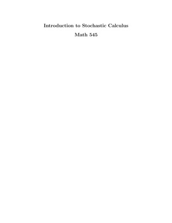
4VALERIE HANLet t denote the time increment and x denote the position change eachtime increment. (The position change above is 1.) Suppose t 1/N , and Bn t x(X1 · · · Xn ). What happens when N grows very large and x becomessmall?The graph of Bn t against t begins to look like the graph of a continuous funcSNapproachestion. Moreover, by the Central Limit Theorem, the distribution of Nthe standard normal distribution. Both of these qualities are qualities of Brownianmotion.In fact, it can be shown that Brownian motion is the limit of random walks, butthe proof is complicated. The interested reader is encouraged to read the proofof Theorem 5.22 in [4]. This fact legitimizes the intuition that Brownian motionand random walk have similar properties. Moreover, in order to simulate Brownianmotion, one must simulate random walks as we have done here with time and spaceincrements being very small.4. Brownian MotionBrownian motion is one of the most commonly used stochastic processes. It isused to model anything from the random movement of gas molecules to the often(seemingly) random fluctuations of stock prices.In order to model random continuous motion, we define Brownian motion asfollows. For simplicity, we only discuss standard Brownian motion.Definition 4.1. A stochastic process {Bt } is a (standard) Brownian motion withrespect to filtration {Ft } if it has the following three properties:(i) For s t, the distribution of Bt Bs is normal with mean 0 and variancet s. We denote this by Bt Bs N (0, t s).(ii) If s t, the random variable Bt Bs is independent of Fs .(iii) With probability one, the function t 7 Bt is a continuous function of t.Brownian motion is often depicted as, and understood as, a sample path, as inFigure 1(A). However, Figure 1(B) depicts the random nature of the random variable Bt , exposing the hidden ω in Bt (ω). The density of the sample paths gives asense of Brownian motion’s normal distribution, as well as showing that, like therandom walk, the paths of Brownian motion spread out the further they are fromt 0.It may not be clear from the definition why (or if) Brownian motion exists. Infact, Brownian motion does exist. We can show this by first defining the process{Bt } for the dyadic rationals t. After proving that with probability one the functiont 7 Bt is continuous on the dyadics, we can extend Bt to all real t by continuity.The interested reader can see Section 2.5 of [1] for the full proof and construction.We now introduce a property of Brownian motion that is useful in computing theconditional expectation: the martingale property. Note that the first two propertiesin the definition of Brownian motion mean that we can “start over” Brownianmotion at any time t. The value Bt for s t does not depend on knowing theprevious values Br where r s, and the distribution of Bt , given the value ofBs , is identical except shifted vertically by the value Bs . The martingale propertypartially captures this characteristic. Given the stream of information up to time s,
AN INTRODUCTION TO STOCHASTIC CALCULUS(a) A realization of Brownian motion.5(b) Multiple (differentlycolored) realizations ofBrownian motion.Figure 1. Brownian motion simulated with random walk as described in Section 3, adopted from [7].the best guess of any future value of a martingale is precisely the random variable’svalue at time s.Definition 4.2. Let {Mt } be a process adapted to filtration {Ft } such thatE[Mt ] . The process {Mt } is a martingale with respect to {Ft } if for eachs t, E(Mt Fs ) Ms .Remark 4.3. If no filtration is specified, we assume that the filtration is the onegenerated by {Ms : s t}.Definition 4.4. A martingale Mt is a continuous martingale if with probabilityone the function t 7 Mt is continuous.Proposition 4.5. Brownian motion is a continuous martingale.Proof. The function t Bt is continuous with probability one by definition, so allwe need to show is E(Bt Fs ) Bs , which easily follows from the properties ofconditional expectation.E(Bt Fs ) E(Bs Fs ) E(Bt Bs Fs ) by Proposition 2.8(i) Bs E[Bt Bs ] by Proposition 2.8(iii),(iv) Bs since Bt Bs N (0, t s). Now we turn to another property of Brownian motion that is useful in computations and will come into use when proving Ito’s formula in Section 7. While weshall see in Section 5 that Brownian motion has unbounded variation, its quadraticvariation is bounded.Definition 4.6. Let {Xt } be a stochastic process. The quadratic variation of Xtis the stochastic processX 2hXit limXj/n X(j 1)/n .n j tn
6VALERIE HANProposition 4.7. The quadratic variation of Bt is the constant process hBit t.Proof. For ease of notation, we prove the Proposition for t 1. Thus, we want toshow that the variance of hBit is 0 and the expectation is 1.ConsiderQn nX 2Bj/n B(j 1)/n .j 1In order to more easily compute the variance and expected value, we express Qnin terms of a distribution we are familiar with. Let Bj/n B(j 1)/n 2 .Yj 1/ nThen,nQn 1XYj ,n j 1and the random variables Y1 , . . . , Yn are independent, each with distribution Z 2 ,where Z is the standard normal distribution. Thus, E[Yj ] E[Z 2 ] 1, E[Yj2 ] E[Z 4 ] 3, and Var[Yj ] E[Yj2 ] E[Yj ]2 3 1 2.We can now easily calculate the expectation and variance of Qn .nE[Qn ] Var[Qn ] 1XE[Yj ] 1.n j 1n21 XVar[Yj ] .n2 j 1nThus,E[hBit ] lim E[Qn ] 1, andn Var[hBit ] lim Var[Qn ] 0,n as desired. Remark 4.8. Informally, this Proposition tells us that the squared difference of thevalues of Brownian motion on a small interval is just the length of the interval.This gives us the intuition (dBt )2 dt, which is often used in stochastic integralcalculations.5. Motivating the Stochastic IntegralIn Section 4, we discussed some of the properties that make Brownian motioneasy to work with. In contrast, the property we discuss in this section is the nondifferentiability of Brownian motion.Theorem 5.1. With probability one, the function t Bt is nowhere differentiable.Remark 5.2. Note that this is stronger than the statement “For every t, the derivative does not exist at t with probability one.”
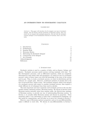
AN INTRODUCTION TO STOCHASTIC CALCULUS7Rather than including a formal proof of this fact, which is located in manydifferent places (e.g. see proof of Theorem 2.6.1 in [1]), we give a more intuitiveexplanation for why this fact should not be surprising. BsSuppose Bt were differentiable at time s. Then, the limit limt s Btt swouldexist, so both the right and left hand limits would exist and be equal. However,this would mean that knowing Br for 0 r s would tell us something aboutBs t Bs for t sufficiently small, which seemingly contradicts with the factthat Bs t Bs is independent of the information given by Br for r s.The non-differentiability of Brownian motion also implies that Brownian motionhas unbounded variation (see Corollary 25 in [5]), which means we cannot simplyuse the Riemann-Stieltjes integral to define an integral with respect to Bt .6. Construction of Ito IntegralAs explained in Section 5, due to Brownian motion’s non-differentiability andunbounded variation,R we cannot simply use Riemann-Stieltjes integration for antintegral of the form 0 As dBs . However, we can use a similar strategy as the oneused to define the Lebesgue integral.Recall that, in the construction of the Lebesgue integral, we first defined theintegral for simple functions and then approximated other, more general, functionswith simple functions. Similarly, for the Ito integral, we first define the integral forsimple processes, and then approximate other functions with simple processes.Definition 6.1. A process At is a simple process if there exist a finite number oftimes 0 t0 t1 · · · tn and associated Ftj -measurable random variablesYj such that At Yj on the associated interval tj t tj 1 . We denote tn 1 .Simple processes, like the simple functions used in the construction of the Lebesgueintegral, are an extension of step functions. Any realization of a simple process lookslike a step function with a finite number of intervals, with the last interval’s right“endpoint” being , as in Figure 2.4 AtY1Y22Y0t12345 Y3 6 2Figure 2. A realization of a simple process At with t0 0, t1 1,t2 2, and t3 5.
8VALERIE HANWe can now define the integral of a simple process, much like how we woulddefine the Riemann-Stieltjes integral. However, unlike with Riemann-Stieltjes integration, where the endpoint chosen does not affect the properties of the integral, theendpoint chosen for the stochastic integral is significant. As we shall see in 6.4, themartingale property of the integral relies on choosing the left endpoint. Moreover,from an intuitive standpoint, given the use of stochastic processes to model realworld systems evolving with time, we may want to only use “past” values, whichcorresponds to the left endpoint, rather than “future” ones.Definition 6.2. Let At be a simple process as in Definition 6.1. Let t 0 suchthat tj t tj 1 . Define the stochastic integral of a simple process to beZ tjXAs dBs Yi (Bti 1 Bti ) Yj (Bt Btj ).0i 0Remark 6.3. More generally, to start integrating from a non-zero time, we defineZ tZ tZ rAs dBs As dBs As dBsr.00This newly defined integral has a number of properties we’d expect from an integral, such as linearity and continuity. However, it also has other useful propertiesthat come into use for computations, as well as for proving Ito’s formula in Section9.Proposition 6.4. Let Bt be a standard Brownian motion with respect to a filtration{Ft }, and let At , Ct be simple processes. Then, the following properties hold.(i) (Linearity) Let a, b R. Then, aAt bCt is also a simple process, andZ tZ tZ t(aAs bCs )dBs aAs dBs bCs dBs .00Moreover, if 0 r t,Z tZAs dBs 00rZAs dBs 0tAs dBs .rRt(ii) (Continuity) With probability one, the function t 7 0 As dBs is a continuous function.Rt(iii) (Martingale) The process Zt 0 As dBs is a martingale with respect to{Ft }.Rt(iv) (Ito isometry) The process Zt 0 As dBs has varianceZ t2Var[Zt ] E[Zt ] E[A2s ]ds.0Proof. Let At be a simple process as in Definition 8.1. Let tj t tj 1 .(i) Linearity easily follows from the definition of a simple process and the definition of the stochastic integralfor simple processes.RtPj(ii) By Definition 8.3, 0 As dBs i 0 Yi (Bti 1 Bti ) Ytj (Bt Btj ). Then,sincethe function t 7 Bt is continuous with probability one, the function t 7 RtAdBss is also continuous with probability one.0(iii) We show E(Zt Fs ) Zs for s t.
AN INTRODUCTION TO STOCHASTIC CALCULUS9Let s t. We only consider the case of s tj and t tk , where the meat of theargument lies. (Note that since s t, j k.)Then, we havek 1XZt Zs Yi [Bti 1 Bti ].i jWe will now use the properties of conditional expectation to compute E(Zt Fs ).E(Zt Fs ) E(Zs Fs ) k 1XE(Yi [Bti 1 Bti ] Fs ) by Proposition 2.8(i)i j Zs k 1XE(Yi [Bti 1 Bti ] Fs ) by Proposition 2.8(iii)i jConsider the sum. Since j i k 1, ti s. Hence, by Proposition 2.8(ii),each term of the sum can be expressed asE(Yi [Bti 1 Bti ] Fs ) E(E(Yi [Bti 1 Bti ] Fti ) Fs ).Recall that Yi is Fti measurable by definition of a simple process and Bti 1 Btiis independent of Fti by definition of Brownian motion.E(Yi [Bti 1 Bti ] Fti ) Yi E(Bti 1 Bti Fti ) by Proposition 2.8(iii) Yi E(Bti 1 Bti ) by Proposition 2.8(iv) 0 since Bti 1 Bti N (0, ti 1 ti ).Thus, all the terms of the sum are 0, giving us E(Zt Fs ) Zs .(iv) We compute Var[Zt ] E[Zt2 ] E[Zt ]2 again using the properties of conditional expectation.We again only consider the case t tj , giving usZt j 1XYi [Bti 1 Bti ] andi 0Zt2 j 1 Xj 1XYi [Bti 1 Bti ]Yk [Btk 1 Btk ].i 0 k 0We first show E[Zt ] 0, which gives us Var[Zt ] E[Zt2 ].E[Zt ] j 1XE[Yi [Bti 1 Bti ]] by linearity of expectationi 0 j 1XE[E(Yi [Bti 1 Bti ] Fti )] by Proposition 2.8(ii)i 0 j 1XE[Yi E([Bti 1 Bti ] Fti )] by Proposition 2.8(iii)i 0 j 1XE[Yi E[[Bti 1 Bti ]]] by Proposition 2.8(iv)i 0 0 since Bti 1 Bti N (0, ti 1 ti ).
10VALERIE HANNow we compute E[Zt2 ]. By linearity of expectation, we haveE[Zt2 ] j 1 Xj 1XE[Yi [Bti 1 Bti ]Yk [Btk 1 Btk ]].i 0 k 0Each term with i k can be expressed asE[Yi [Bti 1 Bti ]Yk [Btk 1 Btk ]] E[E(Yi [Bti 1 Bti ]Yk [Btk 1 Btk ] Ftk )].Note that for i k, Yi , Bti 1 Bti , and Yk are Ftk -measurable, and Btk 1 Btkis independent of Ftk , allowing us to compute the conditional expectation insideeach term.E(Yi [Bti 1 Bti ]Yk [Btk 1 Btk ] Ftk ) Yi [Bti 1 Bti ]Yk E([Btk 1 Btk ] Ftk )by Proposition 2.8(iii) Yi [Bti 1 Bti ]Yk E[[Btk 1 Btk ]]by Proposition 2.8(iv) 0 since Btk 1 Btk N (0, tk 1 tk ).The same argument holds for i k, so we are left withE[Zt2 ] j 1XE[Yi2 (Bti 1 Bti )2 ].i 0By Proposition 2.8(ii), we can express each term asE[Yi2 (Bti 1 Bti )2 ] E[E(Yi2 [Bti 1 Bti ]2 Fti )].Since Yi2 is Fti -measurable and (Bti 1 Bti )2 is independent of Fti , we can againuse the properties of conditional expectation.E(Yi2 [Bti 1 Bti ]2 Fti ) Yi2 E([Bti 1 Bti ]2 Fti ) by Proposition 2.8(iii) Yi2 E[(Bti 1 Bti )2 ] by Proposition 2.8(iv) Yi2 (ti 1 ti ) since E[(Bti 1 Bti )2 ] Var[Bti 1 Bti ].Thus, we have(6.5)E[Zt2 ] j 1XE[Yi2 ](ti 1 ti )i 0Note that the function s 7 E[A2s ] is a step function with the value E[Yi2 ] forRtti s ti 1 . Thus, (6.5) gives us E[Zt2 ] 0 E[A2s ]ds. Now that we have the stochastic integral for simple processes, we consider amore general process. We show that we can approximate bounded processes withcontinuous paths with a sequence of simple processes that are also bounded.Lemma 6.6. Let At be a process with continuous paths, adapted to the filtrationFt , such that there exists C such that with probability one At C for all t.(n)Then there exists a sequence of simple processes At such that for all t,Z t2(6.7)limE[ As A(n)s ]ds 0.n 0
AN INTRODUCTION TO STOCHASTIC CALCULUS11(n)Moreover, with probability one, for all n, t, At C.(n)(n)Proof. We define At as a simple process approximation of At by letting At R j/nA(j, n) for nj t j 1n , where A(0, n) A0 and A(j, n) n (j 1)/n As ds.(n)Note that by construction, At(n) At C.R 1 (n)Let Yn 0 [At At ]2 dt.are simple processes, and with probability one(n)Note that At is essentially a step function approximation to At , which is con(n)tinuous with probability one, so At At . Then, by the bounded convergencetheorem applied to Lebesgue measure, limn Yn 0.Since the random variables Yn are uniformly bounded, Z 1(n)2[At At ] dt lim E[Yn ] 0.lim En n 0 Given the Lemma, we can now define the stochastic integral of bounded processeswith continuous paths in terms of the integrals of simple processes. Fortunately,because of the constructive nature of the proof, we can actually find the sequencedescribed in the Lemma and not merely know that it exists.(n)Definition 6.8. Let At and At be as in Lemma 8.7. DefineZ tZ tAs dBs limAs(n) dBs .0n 0The same properties as those in Proposition 6.4 hold because all the propertiesare preserved under L2 limits. See proof of Proposition 3.2.3 in [1] for the full proof.Remark 6.9. This definition easily extends to piecewise continuous paths. Let t 0.If As has discontinuities at 0 t0 t1 · · · tn t, then we can defineZ tZ t1Z t2Z tAs dBs As dBs As dBs · · · As dBs .00t1tnSimilarly, to Lebesgue integration, we can extend the definition of the stochasticintegral to unbounded processes, by pushing the bounds further and further andthen taking the limit. Suppose At is an unbounded adapted process with continuouspaths. We have two options. The option that may seem more straightforward iscutting off everything above C on At , such that it becomes bounded by C, andthen taking the limit as C . This is the approach that is often taken forconstructing the Lebesgue integral. For example, see Chapter 2 of [6]. However,the intuition for stochastic integral is different. Since stochastic integrals model aquantity evolving with time, we instead want to “stop time” at a certain point T ,and then take the limit as T . Note that we still have the upper bound on Atmonotonically increasing.Definition 6.10. Let As be adapted with continuous paths. For each n N, let(n)Tn min{t : At n}, and let As As Tn , where s Tn min{s, Tn }. DefineZ tZ t(6.11)As dBs limAs(n) dBs.0n 0
12VALERIE HANBy making the path have the constant value n after time Tn , we have “stopped”(n)the process and obtained bounded, continuous processes As . Thus, the integralR t (n)As dBs is well defined.0Moreover, the limit in (6.11) is also well-defined, as we shall now show.Let Kt max0 s t As , which exists because [0, t] is compact and As is continuous.(n)Then, for all n Kt , As is bounded by Kt for 0 s t, so As As forRtR t (n)0 s t. Thus, 0 As dBs 0 As dBs for n Kt , so the limit is well-defined.Note that Kt is a random variable that depends on the path. Although the otherthree properties hold, this integral may not satisfy the martingale property. (SeeSection 4.1 in [1] for more details.)7. Ito’s FormulaNow that we’ve defined the stochastic integral, we might wonder if there existsa stochastic calculus analogue to the Fundamental Theorem of Calculus. Indeed,there is: Ito’s formula.Theorem 7.1. (Ito’s formula I) Suppose f is a C 2 function. Then for every t,ZZ t1 t 00f (Bs )ds(7.2)f (Bt ) f (B0 ) f 0 (Bs )dBs 2 00Alternatively, we can write1(7.3)df (Bt ) f 0 (Bt )dBt f 00 (Bt )dt2Remark 7.4. Ito’s formula is also called the chain rule of stochastic calculus, referencing the differential form (7.3).Proof. This proof omits some of the technical details in favor of focusing on thebigger ideas. See the proof of Theorem 3.3.1 in [1] for a similar proof with thetechnical details added. Alternatively, for an even more technical proof, see proofof Theorem 8.6.1 in [2] for a different proof.For ease of notation, we prove the Theorem for t 1. Consider f (B1 ) f (B0 ).First write this as the telescoping sumnX(7.5)f (B1 ) f (B0 ) f (Bj/n ) f (B(j 1)/n )j 1so that we can examine the infinitesimal changes in f as well as put it in a formthat is closer to the stochastic integral of a simple process.Now let us look at the second-order Taylor expansion for each term in the sum.Ordinarily, for normal calculus, the second-order term goes to 0, but because of theadded randomness, this does not happen here.Let j,n Bj/n B(j 1)/n . Then, the second-order Taylor expansion gives us1(7.6) f (Bj/n ) f (B(j 1)/n ) f 0 (B(j 1)/n ) j,n f 00 (B(j 1)/n ) 2j,n o( 2j,n ).2Since (7.5) and (7.6) hold for all n N, we have that f (B1 ) f (B0 ) is the sumof the following three limitsnX(7.7)limf 0 (B(j 1)/n ) j,n ,n j 1
AN INTRODUCTION TO STOCHASTIC CALCULUS13nX1limf 00 (B(j 1)/n ) 2j,n , and2 n j 1(7.8)(7.9)limn nXo( 2j,n )j 1The first limit is justR 1a 0simple process approximation to a stochastic integral.Thus, (7.7) is equal to 0 f (Bt )dBt .The third limit is actually just the quadratic variation, and so we have that (7.9)is limn o(1) 0.Now consider the second limit. Comparing withR 1 the statement of the Theorem,we can see that we’d like to show that (7.8) is 21 0 f 00 (Bt )dt.Recall again the quadratic variation. Note that if we could somehow pull f 00 (B(j 1)/n )out of the sum, the limit of the sum would again be the quadratic variation. Yet,the second derivative need not be constant, so we cannot quite do that. However,because f is C 2 , we can approximate f 00 by a step function, which allows us to dothis trick on the intervals where the step function is constant.Call f 00 (Bt ) h(t). Since h is continuous, we can approximate h(t) by the stepfunction h (t) such that for all t, h(t) h (t) .On each interval where h is constant, we can pull out h , leaving us with aRiemann sum. Thus, by the linearity of the Riemann integral, we getZn1X1 1h ((j 1)/n) 2j,n h (t)dt.2 j 12 0Now we show that the sums with h and h are sufficiently close. This is easy toshow because of how how we defined h .nnXX[h(t) h (t)] 2j,n 2j,n .j 1j 1Thus, we have ZnX2 h (t) j,n limlim lim 0n 0j 1giving us that (7.8) is12R101Zh (t)dt 01Zh(t)dt 01f 00 (Bt )dt,0f 00 (Bs )ds, as desired. We give an example that emphasizes the difference between the Ito integral andthe normal calculus integral.Example 7.10. Let f (x) x2 . Then, f 0 (x) 2x and f 00 (x) 2. Thus,Z tZ1 t 00Bt2 B02 f 0 (Bs )dBs f (Bs )ds by Ito’s formula2 00ZZ t1 t2Bs dBs 2ds 0 2 00Z t 2Bs dBs t,0
14VALERIE HANgiving usZt1 2[B t].2 t0Note that this is different from what we might naively expect without seeingIto’s formula, as normal calculus would have us incorrectly guessZ t1Bs dBs Bt2 .20Bs dBs Ito’s formula also has other more general forms. We state one of these here. Theinterested reader is encouraged to read Theorem 3.4.2 and 3.4.3 in [1] for two evenmore general versions.Theorem 7.11. (Ito’s formula II) Suppose f (t, x) is a function that is C 1 in t andC 2 in x. Then for every t, Z t Z t f1 2f f(s, Bs )dBs (s, Bs ) (s, Bs ) ds(7.12) f (t, Bt ) f (0, B0 ) s2 x200 xAgain, we can also write this as(7.13)df (t, Bt ) f f1 2f(s, Bs )dBs (s, Bs ) (s,B)dss x s2 x2The proof is similar to Ito’s formula I, except that the Taylor expansion gives usanother term. See the proof of Theorem 3.4.2 in [1] for more details.We end with an example that uses Ito’s formula II, this time using the differentialform of Ito’s formula.Example 7.14. Let f (t, x) eat bx . Then,2 f x2 (t, x) f t (t, x) af (t, x), f x (t, x) bf (t, x),2and b f (t, x).Let Xt f (t, Bt ) eat bBt . Then, f f1 2f(s, Bs ) ds by Ito’s formula IIdXt (s, Bs )dBs (s, Bs ) x s2 x2 b2 bXt dBt a Xt dt.2AcknowledgmentsI’d like to thank my mentor Yucheng Deng for answering my questions and reviewing my paper. I would also like to thank Abhimanyu Choudhary for helping meunderstand filtrations. Finally, I’d like to thank Professor Peter May for organizingthe program.References[1] Gregory Lawler. Stochastic Calculus: An Introduction with Applications. 2014.[2] Rick Durret
Stochastic calculus is used in a number of elds, such as nance, biology, and physics. Stochastic processes model systems evolving randomly with time. Un- . (ii)For every F t-measurable event A, E[E(X jF t)1 A] E[X1 A], where 1 denotes the indicator function. Notation 2.7. We distinguish conditional expectation from expectation by denot-