Transcription
Introduction to Binary Logistic RegressionDale BergerEmail: dale.berger@cgu.eduWebsite: http://wise.cgu.eduPageContents2How does logistic regression differ from ordinary linear regression?3Introduction to the mathematics of logistic regression4How well does a model fit? Limitations4Comparison of binary logistic regression with other analyses5Data screening6One dichotomous predictor:11156Chi-square analysis (2x2) with Crosstabs8Binary logistic regressionOne continuous predictor:11t-test for independent groups12Binary logistic regressionOne categorical predictor (more than two groups)15Chi-square analysis (2x4) with Crosstabs17Binary logistic regression21Hierarchical binary logistic regression w/ continuous and categorical predictors23Predicting outcomes, p(Y 1) for individual cases24Data source, reference, presenting results25Sample results: write-up and table26How to graph logistic models with Excel27Plot of actual data for comparison to model28How to graph logistic models with SPSS1607Introduction to Binary Logistic Regression1
How does Logistic Regression differ from ordinary linear regression?Binary logistic regression is useful where the dependent variable is dichotomous (e.g., succeed/fail, live/die,graduate/dropout, vote for A or B). For example, we may be interested in predicting the likelihood that anew case will be in one of the two outcome categories.Why not just use ordinary regression?The model for ordinary linear regression (OLS) isYi Bo B1Xi erroriSuppose we are interested in predicting the likelihood that an individual is a female based on body weight.Using real data from 190 Californians who responded to a survey of U.S. licensed drivers (Berger et al.,1990), we could use WEIGHT to predict SEX (coded male 0, female 1). An ordinary least squaresregression analysis tells us that Predicted SEX 2.081 - .01016 * (Body Weight) and r -.649, t(188) -11.542, p .001. A naïve interpretation is that we have a great model.It is always a good idea to graph data to make sure models are appropriate. A scatter plot gives usintraocular trauma! The linear regression model clearly is not appropriate.1.2Weight1001502002501.0.8predicted SEX1.065.557.049-.459.6For someone who weighs 150 pounds, thepredicted value for SEX is .557. Naively,one might interpret predicted SEX as theprobability that the person is a female.Sex M 0 F 1.4.20.0-.250100150200BODY WEIGHT OF RESPONDENT250300However, the model can give predictedvalues that exceed 1.000 and or are lessthan zero, so the predicted values are notprobabilities.The test of statistical significance is based on the assumption that residuals from the regression line arenormally distributed with equal variance for all values of the predictor. Clearly, this assumption is violated.The tests of statistical significance provided by the standard OLS analysis are erroneous.A more appropriate model would produce an estimate of the population average of Y for each value of X.In our example, the population mean approachs SEX 1 for smaller values of WEIGHT and it approachesSEX 0 for larger values of WEIGHT. As shown in the next figure, this plot of means is a curved line. Thisis what a logistic regression model looks like. It clearly fits the data better than a straight line when the Yvariable takes on only two values.Introduction to Binary Logistic Regression2
1.21.0.8.6Sex M 0 F 1.4.20.0-.250100150200250300BODY WEIGHT OF RESPONDENTIntroduction to the mathematics of logistic regressionLogistic regression forms this model by creating a new dependent variable, the logit(P). If P is theprobability of a 1 at for given value of X, the odds of a 1 vs. a 0 at any value for X are P/(1-P). The logit(P)is the natural log of this odds ratio.Definition : Logit(P) ln[P/(1-P)] ln(odds).This looks ugly, but it leads to a beautiful model.In logistic regression, we solve for logit(P) a b X, where logit(P) is a linear function of X, very muchlike ordinary regression solving for Y.With a little algebra, we can solve for P, beginning with the equationln[P/(1-P)] a b Xi Ui.We can raise each side to the power of e, the base of the natural log, 2.71828 This gives us P/(1-P) ea bX. Solving for P, we get the following useful equation:e a bXP 1 e a bXMaximum likelihood procedures are used to find the a and b coefficients. This equation comes in handybecause when we have solved for a and b, we can compute P.This equation generates the curved function shown above, predicting P as a function of X. Using thisequation, note that as a bX approaches negative infinity, the numerator in the formula for P approacheszero, so P approaches zero. When a bX approaches positive infinity, P approaches one. Thus, the functionis bounded by 0 and 1 which are the limits for P.Logistic regression also produces a likelihood function [-2 Log Likelihood]. With two hierarchical models,where a variable or set of variables is added to Model 1 to produce Model 2, the contribution of individualvariables or sets of variables can be tested in context by finding the difference between the [-2 LogLikelihood] values. This difference is distributed as chi-square with df (the number of predictors added).The Wald statistic can be used to test the contribution of individual variables or sets of variables in a model.Wald is distributed according to chi-square.Introduction to Binary Logistic Regression3
How well does a model fit?The most common measure is the Model Chi-square, which can be tested for statistical significance. This isan omnibus test of all of the variables in the model. Note that the chi-square statistic is not a measure ofeffect size, but rather a test of statistical significance. Larger data sets will generally give larger chi-squarestatistics and more highly statistically significant findings than smaller data sets from the same population.A second type of measure is the percent of cases correctly classified. Be aware that this number can easilybe misleading. In a case where 90% of the cases are in Group(0), we can easily attain 90% accuracy byclassifying everyone into that group. Also, the classification formula is based on the observed data in thesample, and it may not work as well on new data. Finally, classifications depend on what percentage ofcases is assumed to be in Group 0 vs. Group 1. Thus, a report of classification accuracy needs to beexamined carefully to determine what it means.A third type of measure of model fit is a pseudo R squared. The goal here is to have a measure similar to Rsquared in ordinary linear multiple regression. For example, pseudo R squared statistics developed by Cox& Snell and by Nagelkerke range from 0 to 1, but they are not proportion of variance explained.LimitationsLogistic regression does not require multivariate normal distributions, but it does require randomindependent sampling, and linearity between X and the logit. The model is likely to be most accurate nearthe middle of the distributions and less accurate toward the extremes. Although one can estimate P(Y 1) forany combination of values, perhaps not all combinations actually exist in the population.Models can be distorted if important variables are left out. It is easy to test the contribution of additionalvariables using hierarchical analyses. However, adding irrelevant variables may dilute the effects of moreinteresting variables. Multicollinearity will not produce biased estimates, but as in ordinary regression,standard errors for coefficients become larger and the unique contribution of overlapping variables maybecome very small and hard to detect statistically.More data is better. Models can be unstable when samples are small. Watch for outliers that can distortrelationships. With correlated variables and especially with small samples, some combinations of valuesmay be very sparsely represented. Estimates are unstable and lack power when based on cells with smallexpected values. Perhaps small categories can be collapsed in a meaningful way. Plot data to assure that themodel is appropriate. Are interactions needed? Be careful not to interpret odds ratios as risk ratios.Comparisons of logistic regression to other analysesIn the following sections we will apply logistic regression to predict a dichotomous outcome variable. Forillustration, we will use a single dichotomous predictor, a single continuous predictor, a single categoricalpredictor, and then apply a full hierarchical binary logistic model with all three types of predictor variables.We will use data from Berger et al. (1990) to model the probability that a licensed American driver drinksalcoholic beverages (at least one drink in the past year). This data set is available as an SPSS.SAV filecalled DRIVER.SAV or from Dale.Berger@cgu.edu .Introduction to Binary Logistic Regression4
Data ScreeningThe first step of any data analysis should be to examine the data descriptively. Characteristics of the datamay impose limits on the analyses. If we identify anomalies or errors we can make suitable adjustments tothe data or to our analyses.The exercises here will use the variables age, marst (marital status), sex2, and drink2 (Did you consumeany alcoholic beverage in the past year?). We can use SPSS to show descriptive information on thesevariables.FREQUENCIES VARIABLES age marst sex2 drink2/STATISTICS STDDEV MINIMUM MAXIMUM MEAN MEDIAN SKEWNESS SESKEW KURTOSIS SEKURT/HISTOGRAM/FORMAT LIMIT(20)/ORDER ANALYSIS.This analysis reveals that we have complete data from 1800 cases for sex2 and drink2, but 17 casesmissing data on age and 10 cases missing data on marst.To assure that we use the same cases for all analyses, we can filter out those cases with any missing data.Under Data, Select cases, we can select cases that satisfy the condition (age 0 & marst 0).Now when we rerun the FREQUENCIES analysis, we find complete data from 1776 on all four variables.We also note that we have reasonably large samples in each subgroup within sex, marital status, anddrink2, and age is reasonably normally distributed with no outliers.We have an even split on sex with 894 males and 882 females. For marital status, there are 328 single, 1205married or in a stable relationship, 142 divorced or separated, and 101 widowed. Overall, 1122 (63.2%)indicated that they did drink in the past year. Coding for sex2 is male 0 and female 1, and for drink2none 0 and some 1.Introduction to Binary Logistic Regression5
One dichotomous predictor: Chi-square compared to logistic regressionIn this demonstration, we will use logistic regression to model the probability that an individual consumedat least one alcoholic beverage in the past year, using sex as the only predictor. In this simple situation, wewould probably choose to use crosstabs and chi-square analyses rather than logistic regression. We willbegin with a crosstabs analysis to describe our data, and then we will apply the logistic model to see how wecan interpret the results of the logistic model in familiar terms taken from the crosstabs analysis. UnderStatistics in Crosstabs, we select Chi-square and Cochran’s and Mantel-Haenszel statistics. Under Cells we select Observed, Column percentages, and both Unstandardized and Standardized residuals. UnderFormat select Descending to have the larger number in the top row for the crosstab display.*One dichotomous predictor - first use crosstabs and chi-square.CROSSTABS/TABLES drink2 BY sex2/FORMAT DVALUE TABLES/STATISTICS CHISQ CMH(1)/CELLS COUNT COLUMN RESID SRESID/COUNT ASIS.Crosstabsdrink2 Did you drink last year? * sex2 Sex M 0 F 1 Crosstabulationsex2 Sex M 0 F 10 Maledrink2 Did you1 Yesdrink last year?Count524112266.9%59.4%63.2%33.2-33.2Std. 3.2Std. sidual% within sex2 Sex M 0 F 1ResidualTotalTotal598% within sex2 Sex M 0 F 10 No1 Female% within sex2 Sex M 0 F 1Overall,63.2% ofrespondentsdid drink atleast onealcoholicbeverage inthe past year.We see that the proportion of females who drink is .594 and the proportion of males who drink is .669. Theodds that a woman drinks are 524/358 1.464, while the odds that a man drinks are 598/296 2.020. Theodds ratio is 1.464/2.020 .725. The chi-square test in the next table shows that the difference in drinkingproportions is highly statistically significant. Equivalently, the odds ratio of .725 is highly statisticallysignificantly different from 1.000 (which would indicate no sex difference in odds of drinking).Introduction to Binary Logistic Regression6
Likelihood ratioChi-square testof independence 10.690(NOT anodds ratio)Alternative toPearson’s chisquareapproximationOddsRatioCalculation of the odds ratio: (524 / 358) / (598 / 296) .725 or the inverse 1 / .725 1.379The odds that women drink are .725 times the odds that men drink; The odds that men drink are 1.4 timesthe odds that women drink. This is not the same as the ratio of probabilities of drinking, where .669 / .594 1.13. From this last statistic, we could also say that the probability of drinking is 13% greater for men.However, we could also say that the percentage of men who drink is 7.5% greater than the percentage ofwomen who drink (because 66.9% - 59.4% 7.5%). Interpret and present these statistics carefully,attending closely to how they are computed, because these statistics are easily confused.Introduction to Binary Logistic Regression7
One dichotomous predictor in binary logistic regressionNow we will use SPSS binary logistic regression to address the same questions that we addressed withcrosstabs and chi-square: Does the variable sex2 predict whether someone drinks? How strong is the effect?In SPSS we go to Analyze, Regression, Binary logistic and we select drink2 as the dependent variableand sex2 as the covariate. Under Options I selected Classification Plots. I selected Paste to save the syntaxin a Syntax file. Here is the syntax that SPSS created, followed by selected output.LOGISTIC REGRESSION VAR drink2/METHOD ENTER sex2/CLASSPLOT/CRITERIA PIN(.05) POUT(.10) ITERATE(20) CUT(.5) .Logistic RegressionAlways check thenumber of cases toverify that you havethe correct sample.Check the coding to assure that youknow which way is up.sex2 is coded Male 0, Female 1Block 0: Beginning BlockBecause more than 50% ofthe people in the samplereported that they did drinklast year, the best predictionfor each case (if we have noadditional information) isthat the person did drink.We would be correct 63.2%of the time, because 63.2%(i.e., 1122 of the 1776people) actually did drink.Introduction to Binary Logistic Regression8
Drinker : Nondrinker ratio1122 / 654 1.716(odds of drinking)B .540; e.540 1.716Pearson Chi-squaretest of independencefrom crosstabs 10.678Block 1: Method EnterLikelihood ratioChi-square test ofindependence(NOT an odds ratio)For comparison:Pearson r -.078, andR squared .006[Note: More than half of both males and females drank some alcohol, so the predicted category foreveryone, both males and females, is still ‘Yes’.]Wald (B/S.E.B)2 (-.322/.099)2 10.650Distributed approximately as chi square with df 1Wald for Sex as the only predictor 10.65.This value is reported in Table 1.Odds Ratio:Odds for females /Odds for males(524/358) / (598/296) 1.464 / 2.020 .725Odds of drinking forGroup 0 (Males) 598 / 296 2.020Introduction to Binary Logistic Regression9
Interpretations: The Wald test for sex is statistically significant, indicating that males are significantly morelikely to drink than females (we can look at the data to see the direction of the effect). The odds that a maledrinks is 2.020, indicating that there are on average 2.020 males who drink for every male who does notdrink. Similarly, there are 1.464 females who drink for every female who does not drink. The ratio of theseodds, computed by dividing the odds of drinking for females (Group 1) by the odds of drinking for males(Group 2) is .725. This complex statistic is often misinterpreted.We can use the logistic regression model to estimate the probability that an individual is in a particularoutcome category. In this simple model we have only one predictor, X1 sex2. We can calculate U Constant B1*X1. For a female (X1 1), U1 .703 (-.322)*(1) .381. We can find an estimate of theprobability that Y 1 (i.e., that she drinks) for a female using the following formula:eUi2.718 .3811.46375ˆYi .594 . Check this result in the crosstab table.Ui.3811 1.463751 e1 2.718Although the logistic model is not very useful for a simple situation where we can simply find theproportion in a crosstab table, it is much more interesting and useful when we have a continuous predictoror multiple predictors.Below is a plot of predicted p(Y 1) for every case in our sample, using only sex2 as a predictor. Thepredicted p(Y 1) is .594 for females and .669 for males. However, because p(Y 1) .50 for all bothmales and females, we predict Y 1 for all cases.Step number: 1Observed Groups and Predicted Probabilities1600 F R1200 E FemalesMalesQ U YY E800 YY N YY C YY Y YY 400 NY NN NN NN Predicted ----------Prob:0.25.5.751Group: YYYYYYYYYYPredicted Probability is of Membership for YesThe Cut Value is .50Symbols: N - NoY - YesEach Symbol Represents 100 Cases.Introduction to Binary Logistic Regression10
One continuous predictor: t-test compared to logistic regressionWhen we have two groups and one reasonably normally distributed continuous variable, we can test for adifference between the group means on the continuous variable with a t-test. For illustration, we willcompare the results of a standard t-test with binary logistic regression with one continuous predictor.In this example, we will use age to predict whether people drank alcohol in the past year.T-TESTGROUPS drink2(0 1)/MISSING ANALYSIS/VARIABLES age/CRITERIA CIN(.95) .T-TestOn average, people who did not drink at all were 47.78 years old, while those who drank at least somealcohol were 38.96 years old. This implies that the odds of drinking are lower for older people. Logisticregression will give us the actual value.The test of statistical significance for age shows t (df 1774) 11.212, clear evidence of a relationshipbetween age and drinking, with older people drinking less, on average. In anticipation of logistic analysiswhere chi-square is used to test the contribution of predictor variables, recall that chi-squared with df 1 isequal to z squared. With df 1000, t is close to z, so we can expect that a chi-square test of the age effectwill be about (10.829) 2 117.Introduction to Binary Logistic Regression11
One continuous predictor in binary logistic regressionHere we will use SPSS binary logistic regression to address the same questions that we addressed with thet-test: Does the variable age predict whether someone drinks? If so, how strong is the effect?In SPSS we go to Analyze, Regression, Binary logistic and we select drink2 as the dependent variableand age as the covariate. I selected Classification Plots under Options. I clicked Paste to save the syntax ina Syntax file. Here is the syntax that SPSS created, followed by selected output.LOGISTIC REGRESSION VAR drink2/METHOD ENTER age/CLASSPLOT/CRITERIA PIN(.05) POUT(.10) ITERATE(20) CUT(.5) .Logistic RegressionBlock 0: Beginning BlockIntroduction to Binary Logistic Regression12
Block 1: Method EnterRecall that the square ofthe t statistic was 117.For comparison,Pearson r -.257, andR squared .066Wald for age as theonly predictor 111.58.This value is reported inTable 1Modeled odds ofdrinking : not drinkingfor someone age 0 is7.118![Model extrapolatedbeyond observed data!]The value of Exp(B) for AGE is .968. This means that the predicted odds of drinking are .968 as great forsomeone who is one year older than a comparison person. Alternatively, the predicted odds of drinking onaverage are (1/.968) 1.033 times greater for a person who is one year younger. This model ignores allother variables and assumes that the log of the odds of drinking is linear with respect to age. We canpredict the probability of drinking for an individual at any age.For someone who is 80 years old, U 1.963 (-.033)(80) -.677.eUi2.718 .677.508ˆY .337The modeled probability of drinking is i1 eUi 1 2.718 .677 1 .508For someone age 21, U 1.270 and predicted probability of drinking .781, or 78.1%.Introduction to Binary Logistic Regression13
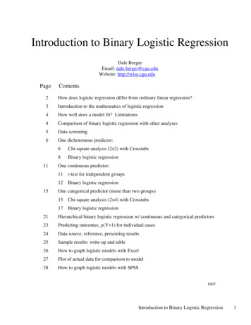
Here is a plot of predicted p(Y 1) for individuals in our sample. The horizontal axis represents age, withyounger people on the right because they have larger predicted probability values (P) compared to olderpeople. This plot is essentially a mirror image of the histogram for age presented earlier.Step number: 1Observed Groups and Predicted Probabilities160 OlderYounger Y Y Y Y F Y YY R120 Y YY E Y YY Q Y YY Y U YYYY Y E80 YYYYYY Y N Y YYYYYYYYY C YYYYYYYYYYYYY Y Y YYYYYY Y YYYYYYYNYYYY 40 Y NYYYYYYYYNYYYYNYNNYYYY YYNYNYNYYYYYYNYYYNNNNNYYYY NYNNNNNNNNNYNNNNNNNNNNNNYNYN YYNNNNNNNNNNNNNNNNNNNNNNNNNNNNN Predicted ---------Prob:0.25.5.751Group: YYYYYYYYYYPredicted Probability is of Membership for YesThe Cut Value is .50Symbols: N - NoY - YesEach Symbol Represents 10 Cases.The default Cut Value is .50. If the estimated P value for an individual is .50 or greater, we predictmembership in the Yes group. Alternatively, we could have set the Cut Value at a lower point because thebase rate for drinking is 63.2%, clearly higher than 50%. Here we could use 1-.632 .368. Then, we wouldpredict that any individual with P of .368 or greater would be a drinker.Consideration of the base rate becomes more important as the base rate deviates farther from .500.Consider a situation where only 1% of the cases fall into the Yes group in the population. We can becorrect 99% of the time if we classify everyone into the No group. We might require extremely strongevidence for a case before classifying it as Yes. Setting the Cut Value at .99 would accomplish that goal.Consideration should be given to the cost and benefits of all four possible outcomes of classification. Is itmore costly to predict someone is a drinker when they are not, or to predict someone is not a drinker whenthey are? Is it more beneficial to classify a drinker as a drinker or to classify a non-drinker as a nondrinker?The UTIL2 program, available on http://wise.cgu.edu , can help one find the optimal Cut Value to maximize‘utility’ of the expected outcome of a classification decision.Introduction to Binary Logistic Regression14
One categorical predictor: Chi-square compared to logistic regressionWhen we have two categorical variables where one is dichotomous, we can test for a relationship betweenthe two variables with chi-square analysis or with binary logistic regression. For illustration, we willcompare the results of these two methods of analysis to help us interpret logistic regression.In this example, we will use marital status to model whether people drank alcohol in the past year.CROSSTABS/TABLES drink2 BY marst/FORMAT AVALUE TABLES/STATISTIC CHISQ/CELLS COUNT COLUMN SRESID.Chi-square with df 1 is a ‘blob’ test.Standardized Residuals (SRESID)provides a cell-by-cell test of deviationsfrom the independence modelCrosstabsThe Standardized Residuals can be tested with z, so a Std. Residual that exceeds 1.96 in absolutevalue can be considered statistically significant with two-tailed alpha .05. These eight tests (onefor each cell) are not independent of each other and of course they depend very much on samplesize as well as effect size. Here we see that compared to expectations (based on independence ofdrinking and marital status), significantly fewer single people were non-drinkers, fewer widowedpeople were drinkers (z -2.9), and more widowed people were nondrinkers (z 3.7).Introduction to Binary Logistic Regression15
Chi-square with df 1 is a ‘blob’ test.The proportion of drinkers is not thesame for all marital status groups, butwe don’t know where the differencesexist or how large they are.The overall tests provided by Pearson Chi-Square and by the Likelihood Ratio Chi-Square indicate that themarital categories differ in the proportions of people who drink. However, these tests are ‘blob’ tests thatdon’t tell us where the effects are or how large they are. The tests of standardized residuals give us morefocused statistical tests, and the proportions who drink in each marital status give us more descriptivemeasures of the effect.From the crosstab table, we see that 70.4% of single people drink, while only 40.6% of widowed peopledrank in the past year. We could also compare each group to the largest group, married, where 62.8% drink.If we were to conduct a series of 2x2 chi-square tests, we would find that single people are significantlymore likely to drink than married people, while widowed people are significantly less likely to drink thanmarried people (we could report 2x2 chi square tests to supplement overall statistics).The odds that a single person drinks is the ratio of those who drink to those who do not drink, 231/97 2.381. The odds that a widowed person drinks is 41/60 .683. Compared to the widowed folks, the oddsthat single people drink is (231/97) / (41/60) 2.381/.683 3.485 times greater.Odds ratios are often misinterpreted, especially by social scientists who are not familiar with odds ratios.Here is a Bumble interpretation: “Single people are over three times more likely to drink than widowedpeople.” This is clearly wrong, because 70.4% of single people drink compared to 40.6% for widowedpeople, which gives 70.4%/40.6% 1.73, not even twice as likely.Important lesson: The odds ratio is not the same as a ratio of probabilities for the two groups.Note the highly significant linear-by-linear association. What does this mean here? Not much – maritalstatus is not even an ordinal variable, much less an interval measure. We just happen to have codedsingle 1 and widowed 4, so the linear-by-linear association is greater than chance because people withlarger scores on marital status are significantly less likely to drink than those with smaller scores, onaverage.How else could you describe the difference between single and widowed people in their drinking? Theproportion of people who drink in each category would be very useful for description.Next we will analyze these same data with binary logistic regression and compare the analyses.Introduction to Binary Logistic Regression16
One categorical predictor (groups 2) with binary logistic regressionHow is marital status related to whether or not people drink? We will use SPSS binary logistic regression toaddress this question and compare findings to our earlier 2x4 chi-square analysis.In SPSS we go to Analyze, Regression, Binary logistic and we select drink2 as the dependent variableand marst as the covariate. Click Categorical to define the coding for marst. “Indicator” coding is alsoknown as ‘dummy’ coding, whereby cases that belong in a certain group (e.g., single) are assigned thevalue of 1 while all others are assigned the value of 0. We need three dummy variables to definemembership in all four groups; SPSS creates these for us automatically. There are many other choices forconstructing contrasts. However we do it, we need (k – 1) contrasts each with df 1 to identifymembership in k groups. Under Options, I selected Classification Plots. I selected Paste to save the syntaxin a Syntax file. Here is the syntax that SPSS created, followed by selected output.LOGISTIC REGRESSION VAR drink2/METHOD ENTER marst/CONTRAST (marst) Indicator/CLASSPLOT/CRITERIA PIN(.05) POUT(.10) ITERATE(20) CUT(.5) .Logistic RegressionCase Processing SummaryUnweighted CasesSelected CasesaNIncluded in Analysis1776100.00.0Missing CasesDependent Variable EncodingPercentOriginal ValueInternal Value0 No01 Yes1dimension0Total1776100.00.01776100.0Unselected CasesTotala. If weight is in effect, see classification table for the total number ofcases.Categorical Variables CodingsParameter codingFrequencymarst MARITAL STATUS1 SINGLE(1)(2)(3)3281.000.000.0001205.0001.000.0003 DIV OR SEP142.000.0001.0004 WIDOWED101.000.000.0002 MARRIED OR STBLCheck this coding carefully. The first parameter is a dummy code (indicator variable)comparing SINGLE vs. all others combined. Groups 2 and 3 are coded similarly.WIDOWED is the reference group that is omitted from this set of coded variables.Introduction to Binary Logistic Regression17
Block 0: Beginning BlockClassification Tablea,bObservedPredictedDid you drink last year?0 NoStep 0Did you drink last year?1 YesPercentageCorrect0 No0654.01 Yes01122100.0Overall Percentage63.2a. Constant is included in the model.b. The cut value is .500For variables not in the model, we have testsfor the contribution that each single variablewould make if it were added to the modelby itself. Thus, we see that MARST(1)(single vs. all others combined) would makea statistically significant contribution (p .003). MARST(2) and MARST(3) wouldnot make significant contributions bythemselves. The Score values are chi-squaretests of the individual variables; these arereported in Table 1 in the sample write-up.Pearson χ2Block 1: Method EnterOmnibus Tests of Model CoefficientsChi-squareStep .000Compare to theLikelihood ratiochi-square fromCROSSTABSLikelihoodratio χ2There is no equivalent r or Rsquared for comparison.Introduction to Binary Logistic Regression18
Wald forMarital Statusas the onlypredictor,reported inTable 1.Individualgroups arecompared tothe referencegr
where a variable or set of variables is added to Model 1 to produce Model 2, the contribution of individual variables or sets of variables can be tested in context by finding the difference between the [-2 Log Likelihood] values. This difference is distributed