Transcription
Introduction to Stochastic CalculusMath 545
ContentsChapter 1. Introduction1. Motivations2. Outline For a Course556Chapter 2. Probabilistic Background1. Countable probability spaces2. Uncountable Probability Spaces3. Distributions and Convergence of Random Variables991118Chapter 3. Wiener Process and Stochastic Processes1. An Illustrative Example: A Collection of Random Walks2. General Stochastic Proceses3. Definition of Brownian motion (Wiener Process)4. Constructive Approach to Brownian motion5. Brownian motion has Rough Trajectories6. More Properties of Random Walks7. More Properties of General Stochastic Processes8. A glimpse of the connection with pdes212122232426282934Chapter 4. Itô Integrals1. Properties of the noise Suggested by Modeling2. Riemann-Stieltjes Integral3. A motivating example4. Itô integrals for a simple class of step functions5. Extension to the Closure of Elementary Processes6. Properties of Itô integrals7. A continuous in time version of the the Itô integral8. An Extension of the Itô Integral9. Itô Processes37373839404446474849Chapter 5. Stochastic Calculus1. Itô’s Formula for Brownian motion2. Quadratic Variation and Covariation3. Itô’s Formula for an Itô Process4. Full Multidimensional Version of Itô Formula5. Collection of the Formal Rules for Itô’s Formula and Quadratic Variation515154586064Chapter 6. Stochastic Differential Equations1. Definitions2. Examples of SDEs3. Existence and Uniqueness for SDEs4. Weak solutions to SDEs67676871743
5.Markov property of Itô diffusions76Chapter 7. PDEs and SDEs: The connection1. Infinitesimal generators2. Martingales associated with diffusion processes3. Connection with PDEs4. Time-homogeneous Diffusions5. Stochastic Characteristics6. A fundamental example: Brownian motion and the Heat Equation77777981848586Chapter 8. Martingales and Localization1. Martingales & Co.2. Optional stopping3. Localization4. Quadratic variation for martingales5. Lévy-Doob Characterization of Brownian-Motion6. Random time changes7. Time Change for an sde8. Martingale representation theorem9. Martingale inequalities8989919295979999100100Chapter 9. Girsanov’s Theorem1. An illustrative example2. Tilted Brownian motion3. Shifting Weiner Measure Simple Cameron Martin Theorem4. Girsanov’s Theorem for sdes103103104105106Bibliography109Appendix A.Some Results from Analysis1114
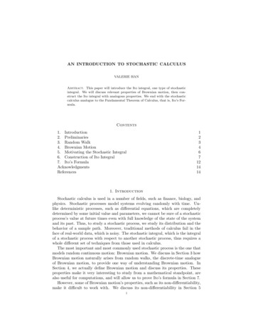
CHAPTER 1Introduction1. MotivationsEvolutions in time with random influences/random dynamics. Let N ptq be the“number of rabbits in some population” or “the price of a stock”. Then one might want to make amodel of the dynamics which includes “random influences”. A (very) simple example isdN ptq“ aptqN ptq where aptq “ rptq “noise” .(1.1)dtMaking sense of “noise” and learning how to make calculations with it is one of the principalobjectives of this course. This will allow us predict, in a probabilistic sense, the behavior of N ptq .Examples of situations like the one introduced above are ubiquitous in nature:i) The gambler’s ruin problem We play the following game: We start with 3 in ourpocket and we flip a coin. If the result is tail we loose one dollar, while if the result ispositive we win one dollar. We stop when we have no money to bargain, or when we reach9 . We may ask: what is the probability that I end up broke?ii) Population dynamics/Infectious diseases As anticipated, (1.1) can be used to modelthe evolution in the number of rabbits in some population. Similar models are used tomodel the number of genetic mutations an animal species. We may also think about N ptqas the number of sick individuals in a population. Reasonable and widely applied models forthe spread of infectious diseases are obtained by modifying (1.1), and observing its behavior.In all these cases, one may be inteested in knowing if it is likely for the disease/mutationto take over the population, or rather to go extinct.iii) Stock prices We may think about a set of M risky investments (e.g. a stock), where theprice Ni ptq for i P t1, . . . M u per unit at time t evolves according to (1.1). In this case, oneřone would like to optimize his/her choice of stocks to maximize the total value Mi“1 αi Ni ptqat a later time T .Connections with diffusion theory and PDEs. There exists a deep connection betweennoisy processes such as the one introduced above and the deterministic theory of partial differentialequations. This starling connection will be explored and expanded upon during the course, but weanticipate some examples below:i) Dirichlet problem Let upxq be the solution to the pde given below with the notedBBboundary conditions. Here “ Bx. The amazing fact is the following: If we start a ByBrownian motion diffusing from a point px0 , y0 q inside the domain then the probabilitythat it first hits the boundary in the darker region is given by upx0 , y0 q.ii) Black Scholes Equation Suppose that at time t “ 0 the person in iii) is offered theright (without obligation) to buy one unit of the risky asset at a specified price S and ata specified future time t “ T . Such a right is called a European call option. How muchshould the person be willing to pay for such an option? This question can be answered bysolving the famous Black Scholes equation, giving for any stock price N ptq the rigth valueS of the European option.5
u 012 u 0u 12. Outline For a CourseWhat follows is a rough outline of the class, giving a good indication of the topics to be covered,though there will be modifications.i) Week 1: Motivation and Introduction to Stochastic Process(a) Motivating Examples: Random Walks, Population Model with noise, Black-Scholes,Dirichlet problems(b) Themes: Direct calculation with stochastic calculus, connections with pdes(c) Introduction: Probability Spaces, Expectations, σ-algebras, Conditional expectations,Random walks and discrete time stochastic processes. Continuous time stochastic processes and characterization of the law of a process by its finite dimensional distributions(Kolmogorov Extension Theorem). Markov Process and Martingales.ii) Week 2-3: Brownian motion and its Properties(a) Definitions of Brownian motion (BM) as a continuous Gaussian process with independent increments. Chapman-Kolmogorov equation, forward and backward Kolmogorovequations for BM. Continuity of sample paths (Kolmogorov Continuity Theorem).BM and more Markov process and Martingales.(b) First and second variation (a.k.a variation and quadratic variation) Application toBM.iii) Week 4: Stochastic Integrals(a) The Riemann-Stieltjes integral. Why can’t we use it ?şt(b) Building the Itô and Stratonovich integrals. (Making sense of “ 0 σ dB.”)(c) Standard propertiesof integralsşş hold: linearity, additivity(d) Itô isometry: Ep f dBq2 “ E f 2 ds.iv) Week 5: Itô’s Formula and Applications(a) Change of variable.(b) Connections with pdes and the Backward Kolmogorov equation.v) Week 6: Stochastic Differential Equations(a) What does it mean to solve an sde ?(b) Existence of solutions (Picard iteration). Uniqueness of solutions.vi) Week 7: Stopping Times(a) Definition. σ-algebra associated to stopping time. Bounded stopping times. Doob’soptional stopping theorem.(b) Dirichlet Problems and hitting probabilities.(c) Localization via stopping timesvii) Week 8: Levy-Doob theorem and Girsonov’s Theorem(a) How to tell when a continuous martingale is a Brownian motion.6
(b) Random time changes to turn a Martingale into a Brownian Motion(c) Hermite Polynomials and the exponential martingale(d) Girsanov’s Theorem, Cameron-Martin formula, and changes of measure.(1) The simple example of i.i.d Gaussian random variables shifted.(2) Idea of Importance sampling and how to sample from tails.(3) The shift of a Brownian motion(4) Changing the drift in a diffusion.viii) Week 9: sdes with Jumpsix) Week 10: Feller Theory of one dimensional diffusions(a) Speed measures, natural scales, the classification of boundary point.7
CHAPTER 2Probabilistic BackgroundExample 0.1. We begin with the following motivating example. Consider a random sequenceω “ tωi uNi“0 where#1 with probability 12ωi “ 1 with probability 21independent of the other ω’s. We will also write this asPrpω1 , ω2 , . . . , ωN q “ ps1 , s2 , . . . , sN qs “12Nfor si “ 1. We can group the possible outcomes into subsets depending on the value of ω1 :F1 “ ttω P Ω : ω1 “ 1u, tω P Ω : ω1 “ 1uu .(2.1)These subsets contain the possible events that we may observe knowing the value of ω1 . In otherwords, this separation represents the information we have on the process at that point.Let Ω be the set of all such sequences of length N (i.e. Ω “ t 1, 1uN ), and consider now thesequence of functions tXn : Ω Ñ Zu whereX0 pωq “ 0nÿXn pωq “ωi(2.2)i“1for n P t1, , N u. Each Xn is an example of an integer-valued random variable. The set Ω iscalled the sample space (or outcome space) and the measure given by P on Ω is called the probabilitymeasure.We now recall some basic definitions from the theory of probability which will allow us to putthis example on solid ground.Intuitively, each ω P Ω is a possible outcome of all of the randomness in our system. Themeasure P gives the chance of the various outcomes. In the above setting where the outcome spaceΩ consists of a finite number of elements, we are able to define everything in a straightforward way.We begin with a quick recalling of a number of definitions in the countably infinite (possibly finite)setting.1. Countable probability spacesIf Ω is countable it is enoughř to define the probability of each element in Ω. That is to say givea function p : Ω Ñ r0, 1s with ωPω ppωq “ 1 and definePrωs “ ppωq9
for each ω P Ω. An event A is just a subset of Ω. We naturally extend the definition of P to anevent A byÿPrAs :“P rωs .ωPAObserve that this definition has a number of consequences. In particular, if Ai are disjoint events,that is to say Ai Ă Ω and Ai X Ak “ H if i ‰ j then«ff88ďÿPAi “PrAi si“1i“1Acand if:“ tω P Ω with ω R Au is the compliment of A then PrAs “ 1 PrAc s.Given two event A and B, the conditional probability of A given B is defined byPrA Bs :“PrA X BsPrBs(2.3)For fixed B, this is just a new probability measure Pr Bs on Ω which gives probability Prω Bs tothe outcome ω P Ω.A real-valued random variable X is simply a real-valued function of Ω. Similarly, a randomvariable taking values in some set X is a function X : Ω Ñ X. We can then define the expected valueof a random variable X (or simply the expectation of X) asÿÿErXs :“xPrX “ xs “XpωqPrωsωPΩxPRangepXqHere we have used the convention that tX “ xu is short hand for tω P Ω : Xpωq “ xu and thedefinition of RangepXq “ tx P X : Dω, with Xpωq “ xu “ X 1 pΩq.Two events A and B are independent if PrA X Bs “ PrAsPrBs. Two random variable areindependent if PrX “ x, Y “ ys “ PrX “ xsPrY “ ys. Of course this implies that for any events Aand B that PrX P A, Y P Bs “ PrX P AsPrY P Bs and that ErXY s “ ErXsErY s. A collection ofevents Ai is said to be mutually independent ifnźPrA1 X X An s “PrAi s .i“1Similarly a collection of random variable Xi are mutually independent if for any collection of setsfrom their range Ai one has that the collection of events tXi P Ai u are mutually independent. Asbefore, as a consequence one has thatnźErX1 . . . Xn s “ErXi s .i“1Given two X-valued random variables Y and Z, for any z P Range(Z) we define the conditionalexpectation of Y given tZ “ zu asÿErY Z “ zs :“yPrY “ y Z “ zs(2.4)yPRangepY qWhich is to say that ErY Z “ zs is just the expected value of Y under the probability measurewhich is given by P r Z “ zs.In general, for any event A we can define the conditional expectation of Y given A asÿErY As :“yPrY “ y As(2.5)yPRangepY q10
We can extend the definition ErY Z “ zs to ErY Zs which we understand to be a function of Z whichtakes the value ErY Z “ zs when Z “ z. More formally ErY Zs :“ hpZq where h : RangepZq Ñ Xgiven by hpzq “ ErY Z “ zs.Example 1.1. Let us compute an example of conditional probability. Using the notation fromExample 0.1 we seeÿErpX3 q2 X2 “ 2s “iPrpX3 q2 “ i X2 “ 2siPN“ p1q2 PrX3 “ 1 X2 “ 2s p3q2 PrX3 “ 3 X2 “ 2s “ 5Of course, X2 can also take the value 2 and 0. For these values of X2 we haveErpX3 q2 X2 “ 2s “p 1q2 PrX3 “ 1 X2 “ 2s p 3q2 PrX3 “ 3 X2 “ 2s “ 5ErpX3 q2 X2 “ 0s “p 1q2 PrX3 “ 1 X2 “ 0s p1q2 PrX3 “ 1 X2 “ 0s “ 1Hence ErpX3 q2 X2 “ 2s “ hpX2 q where#hpxq “51if x “ 2if x “ 0By clever rearrangement one does not always have to calculate the function ErY Zs so explicitly.Consider the following examples.«ff«ff76ÿÿErX7 X6 s “ Eωi X6 “ Eωi ω7 X6i“1i“1“E rX6 ω7 X6 s “ ErX6 F6 s Erω7 F6 s“X6 Erω7 s “ X6since Erω7 s “ 0. We can also do a similar calculation for the previous example.ErX32 X2 s “ ErpX2 ω3 q2 X2 s “ ErX22 2ω3 X2 ω32 X2 s“ ErX22 s 2Erω3 sErX2 s Erω32 s “ X22 1since Erω3 s “ 0 and Erω32 s “ 1. Compare this to the definition of h given above.2. Uncountable Probability SpacesWe will need to consider Ω which have uncountably many points. An example is a uniformpoint drawn from r0, 1s. To handle such settings completely rigorously we need ideas from basicmeasure theory. However if one is willing to except a few formal rules of manipulation, we canproceed with learning basic stochastic calculus without needing to distract ourselves with too muchmeasure theory.A R-valued random variable X is called a continuous random variable if there exists a densityfunction ρ : R Ñ R so thatżbPrX P ra, bss “ρpxqdxafor any ra, bs Ă R. More generally a Rn -valued random variable X is called a continuous randomvariable if there exists a density function ρ : Rn Ñ R so thatż b1ż bnżżPrX P ra, bss “ ρpx1 , . . . , xn q dx1 dxn “ρpxqdx “ρpxqLebpdxqa1anra,bs11ra,bs
śfor any ra, bs “ rai , bi s Ă Rn . The last two expressions are just different ways of writing the samething. Here we have introduced the notation Lebpdxq for the standard Lebesgue measure on Rngiven by dx1 dxn .Analogously to the countable case we define the expectation of a continuos random variablewith density ρ byżErhpXqs “hpxqρpxqdx .RnDefinition 2.1. A real-valued random variable X is Gaussian with mean µ and variance σ 2 ifżpx µq21?PrX P As “e 2σ2 dx .2πσ 2AIf a random variable has this distribution we will write X „ N pµ, σq .If X and Y are Rn -valued and Rm -valued random variables, respectively, then the vector pX, Y qis again a continuous Rnˆm -valued random variable which has a density which is called the jointdensity of X and Y . If Y has density ρY and ρXY is the joint density of X and Y we can defineżρXY px, yqPrX P A Y “ ys “dx .ρY pyqApx,yqHence X given Y “ y is a new continuos random variable with density x ÞÑ ρXYρY pyq for a fixed y.The conditional expectation is defined using this density.While many calculations can be handled satisfactorily at this level, we will soon see that weneed to consider random variables on much more complicated spaces such as the space of real-valuedcontinuous functions on the time interval r0, T s which will be denoted Cpr0, T s; Rq. To give all ofthe details in such a setting would require a level of technical detail which we do not wish to enterinto on our first visit to the subject of stochastic calculus. If one is willing to “suspend a littledisbelief” one can learn the formal rule of manipulation, much as one did when one first learnedregular calculus. The technical details are important but better appreciated after one fist has thebig picture.2.1. Sigma Algebras. To this end, we will introduce the idea of a sigma algebra (usuallywritten σ-algebra or σ-field in [Klebaner]). In Section 1, we defined our probability measures bybeginning with assigning a probability to each ω P Ω. This was fine when Ω was finite or countablyinfinite. When Ω “ r0, 1s as in the case of picking a uniform point from the unit interval, theprobability of any given point must be zero. Otherwise the sum of all of the probabilities would be8 since there are infinitely many points and each of them has the same probability as no point ismore or less likely than another. Formally,ÿPrtxus “ 8 if Prtxus ą 0 .xPr0,1sThis is only the tip of the iceberg. There are many more complicated issues. The solution isto fix a collection of subsets of Ω about which we are “allowed” to ask “what is the probabilityof this event?”. We will be able to make this collection of subsets very large, but it will not, ingeneral, contain all of the subsets of Ω in situations where Ω is uncountable. This collections ofsubsets is called the σ-algebra. The triplet pΩ, F, Pq of an outcome space Ω, a probability measureP and a σ-algebra F is called a Probability Space. For any event A P F, the “probability of thisevent happening” is well defined and equal to PrAs. A subset of Ω which is not in F might nothave a well defined probability. Essentially all of the event you will think of naturally will be in theσ-algebra with which we will work. In light of this, it is reasonable to ask why we bring them up12
at all. It turns out that σ-algebras are a useful way to “encode the information” contained in acollection of events or random variables. This idea and notation is used in many different contexts.If you want to be able to read the literature, it is useful to have a operational understanding ofσ-algebras without entering into the technical detail.Before attempting to convey any intuition or operational knowledge about σ-algebras we givethe formal definitions since they are short (even if unenlightening).Definition 2.2. Given a set Ω, a σ-algebra F is a collection of subsets of Ω such thati) Ω P Fii) A P F ùñ Ac “ ΩzA P Fiii) Given tAn u a countable collection of subsets of F, we haveŤ8i“1 AiP F.In this case the pair pΩ, Fq are referred to as a measurable spaceFor us a σ-algebra is the embodiment of information.Example 2.3. If Ω “ Rn or any subset of it, we talk about the Borel σ-algebra as the σ-algebragenerated by all of the intervals ra, bs with a, b P Ω. This σ-algebra contains essentially any event youwould think about in most all reasonable problems. Using pa, bq, or ra, bq or pa, bs or some mixtureof them makes no difference.Given any collection of subsets G of Ω we can talk about the “σ-algebra generated by G” assimply what we get by taking all of the elements of G and exhaustively applying all of the operationslisted above in the definition of a σ-algebra. More formally,Definition 2.4. Given Ω and F a collection of subsets of Ω, σpF q is the σ-algebra generatedby F . This is defined as the smallest (in terms of numbers of sets) σ-algebra which contains F .Intuitively σpF q represents all of the probability data contained in F .Example 2.5 (Example 0.1 continued). In (2.1) we defined the set F1 as the collection of setsof possible outcomes fixing ω1 . This collection of sets generaties a σ-algebra on Ω, given byF1 :“ tH, Ω, tω P Ω : ω1 “ 1u, tω P Ω : ω1 “ 1uu ,(2.6)representing the information we have on the process knowing ω1 .To complete our measurable space pΩ, Fq into a probability space we need to add a probabilitymeasure. Since we will not build our measure from its definition on individual ω P Ω as we did inSection 1 we will instead assume that it satisfies certain reasonable properties which follow fromthis construction in the countable or finite case. The fact that the following assumptions is all thatis needed would be covered in a measure theoretical probability or analysis class.Definition 2.6. A measure P on a measurable space pΩ, Fq is a probability measure ifi) PrΩs “ 1,ii) PrAc s “ 1 PrAs for all A P F.Ťřiii) Given tAi u a finite collection of pairwise disjoint sets in F, P r ni“1 Ai s “ ni“1 PrAi s ,In this case the triplet pΩ, F, Pq is referred to as a probability spaceDefinition 2.7. If pΩ, Fq and pX, Bq are measurable spaces, then ξ : Ω Ñ X is a X-valuedrandom variable if for all B P B we have ξ 1 pBq P F. In other words, admissible events in X getmapped to admissible events in Ω.13
Given any events A and B in F, we define the conditional probability just as before, namelyPrA Bs “PrA X Bs.PrBsGiven real-valued random variable X on a probabilty space pΩ, F, Pq, we define the expected valueof X in a way analogous to before:żEpXq “XpωqPpdωq .ΩWe will take for granted that this integral makes sense. However, it follows from the general theoryof measure spaces.Definition 2.8. Given a random variable on the probability space pΩ, F, Pq taking values in ameasurable space pX, Bq, we define the σ-algebra generated by the random variable X asσpXq “ σptX 1 pBq B P Buq .The idea is that σpXq contains all of the infomation contained in X. If an event is in σpXq thenwhether this event happens or not is completely determined by knowing the value of the randomvariable X.Example 2.9 (Example 0.1 continued). By definition (2.2), since X1 “ ω1 the σ-algebragenerated by the random variable X1 is σpX1 q “ F1 from (2.6). However, the σ-algebra generatedby X2 “ ω1 ω2 is given byσpX2 q “ tH, Ω, tω P Ω : pω1 , ω2 q “ p1, 1qu, tω P Ω : pω1 , ω2 q “ p 1, 1qu, tω P Ω : ω1 ω2 “ 0uu .Note that this σ-algebra is different than F2 “ σpttw P Ω : pw1 , w2 q “ ps1 , s2 qu : s1 , s2 P t 1, 1uuq .Indeed, knowing the value of X2 is not always sufficient to know the value of ω1 “ X1 . Contrarily,knowing the value of pω1 , ω2 q (contained in F2 ) definitely implies that you know the value of X2 . Inother words, (the information of ) σpX2 q is contained in F2 , concisely σpX2 q Ă F2 .Now compare σpX2 q and σpY q where Y “ X22 . Lets consider three events A “ tX2 “ 2u,B “ tX2 “ 0u, C “ tX2 is evenu. Clearly all three events are in the σ-algebra generated by X2 (i.e.σpX2 q) since if you know that value of X2 then you always know whether the events happen or not.Next notice that B P σpY q since if you know that Y “ 0 then X2 “ 0 and if Y ‰ 0 then X2 ‰ 0.Hence no mater what the value of Y is knowing it you can decide if X2 “ 0 or not. However,knowing the value of Y does not always tell you if X2 “ 2. It does sometimes, but not always. IfY “ 0 then you know that X2 ‰ 0. However if Y “ 4 then X2 could be equal to either 2 or 2.We conclude that A R σpY q but B P σpY q. Since X2 is always even, we do not need to know anyinformation to decide C and it is in fact in both σpX2 q and σpY q. In fact, C “ Ω and Ω is in anyσ-algebra since by definition Ω and the empty set H are always included. Lastly, since wheneverwe know X2 we know Y , it is clear that σpX2 q contains all of the information contained in σpY q.In fact it follows from the defintion and the fact that σpY q Ă σpX2 q. To say that one σ-algebra iscontained in another is to say that the second contains all of the information of the first and possiblymore.Definition 2.10. We say that a real-valued random variable X is measurable with respect toσ-algebra G if every set of the form X 1 pra, bsq is in G.11If X is a random variable taking values in a measurable space pX, Bq (recall that B is a σ-algebra over X) thenwe require that X 1 pBq P G for all B P B.14
Speaking intuitively, a random variable is measurable with respect to a given σ-algebra if theinformation in the σ-algebra is always sufficient to fix the value of the random variable. Of coursethe random variable X is always measurable with repect to σpXq. More specifically, σpXq is thesmallest σ-algebra G on Ω such that X is G-measureable. In the previous example, Y is measurablewith respect to σpX2 q since knowing the value of X2 fixes the value of Y .Definition 2.11. If a random variable X is measurable with respect to a σ-algebra F then wewill write X P F. While this is a slight abuse of notation, it will be very convenient.Example 2.12. Let X be a random variable taking values in r 1, 1s. Let g be the function fromr 1, 1s Ñ t 1, 1u such that gpxq “ 1 if x ď 0 and gpxq “ 1 if x ą 0. Define the random variableY by Y pωq “ gpXpωqq. Hence Y is a random variable talking values in t 1, 1u. Let FY be theσ-algebra generated by the random variable Y . That is FY “ σpY q :“ tY 1 pBq : B P BpRqu. In thiscase, we can figure out exactly what FY looks like. Since Y takes on only two values, we see that forany subset B in BpRq(the Borel σ-algebra of R) 1’’Y p 1q :“ tω : Y pωq “ 1u if 1 P B, 1 R B’’’’’if 1 P B, 1 R B&Y 1 p1q :“ tω : Y pωq “ 1u 1Y pBq “’Hif 1 R B, 1 R B’’’’’’if 1 P B, 1 P B%ΩThus FY consists of exactly four sets, namely tH, Ω, Y 1 p 1q, Y 1 p1qu. For a function f : Ω Ñ Rto be measurable with respect the σ-algebra FY , the inverse image of any set B P BpRq must be oneof the four sets in FY . This is another way of saying that f must be constant on both Y 1 p 1q andY 1 p1q. Note that together Y 1 p 1q Y Y 1 p1q “ Ω.We now re-examine the idea of a conditional expectation of a random variable with respect to aσ-algebra. To do so, we introduce the indicator function.Definition 2.13. Given pΩ, F, Pq a probability space and A P F, the indicator function of A is#1 xPA1A pxq “(2.7)0 otherwiseand is a measurable function. Fixing a probability space pΩ, F, Pq, we haveProposition 2.14. If X is a random variable on pΩ, F, Pq with Er X s ă 8, and G Ă F is aσ-algebra, then there is a unique random variable Y on pΩ, G, Pq such thati) Er Y s ă 8 ,ii) Er1A Y s “ Er1A Xs for all A P G .Definition 2.15. We define the conditional expectation with respect to a σ-algebra G as theunique random variable Y from Proposition 2.14, i.e., ErX Gs :“ Y .The intuition behind Proposition 2.15 is that the conditional expectation wrt a σ-algebraG Ă F of a random variable X P F is that random variable Y P G that is equivalent or identical (interms of expected value, or predictive power) to X given the information contained in G. In otherwords, Y “ ErX Gs is the best approximation of the value of X given the information in G. Theprevious definition of conditional expectation wrt a fixed set of events is obtained by evaluating15
the random variable ErX Gs on the events of interest, i.e., by fixing the events in G that may haveoccurred.When we condition on a random variable we are really conditioning on the information thatrandom variable is giving to us. In other words, we are conditioning on the σ-algebra generated bythat random variable:E rX Zs :“ E rX σpZqs .As in the discrete case, one can show that there exists a function h : RangepZq Ñ X such thatErY Zpωqs :“ hpZpωqq ,and hence we can think about the conditional expectation as a function of Zpωq. In particular, thisallows to defineErY Z “ zs :“ hpzq .Example 2.16. When the set Ω is countable, we can write every random variable Y on Ω asÿY pωq “y1Y “y pωq .yPRangepY qConsequently, writingÿErX Z “ zs1Z“z pωq ,ErX Zspωq “zPRangepZqwe obtainEr1Z“z pωqXpωqs “ E r1Z“z pωqErX Z “ zss “ ErX Z “ zs Er1Z“z pωqsNow, recognizing that Er1A s “ PrAs, if PrZ “ zs ‰ 0 we finally obtainÿEr1Z“z pωqXpωqsxPrZ “ z, X “ xsErX Z “ zs ““,PrZ “ zsPrZ “ zsxPRangepXqand recover (2.4).We now list some properties of the conditional expectation:‚ Linearity: for all α, β P R we haveErαX βY Gs “ αErX Gs βErY Gs ,‚ if X is G-measurable thenErXY Gs “ XErY Gs .Intuitively, since X P G (X is measurable wrt the σ-algebra G), the best approximation ofX on the sets contained in G is X itself, so we do not need to approximate it.‚ Tower property: if G and H are both σ-algebras with G Ă H, thenE rE rX Hs Gs “ E rE rX Gs Hs “ E rX Gs .Since G is a smaller σ-algebra, the functions which are measurable with respect to it arecontained in the space of functions measurable with respect to H. More intuitively, beingmeasure with respect to G means that only the information contained in G is left freeto vary. E rE rX Hs Gs means first give me your best guess given only the informationcontained in H as input and then reevaluate this guess making use of only the informationin G which is a subset of the information in H. Limiting oneself to the information in G isthe bottleneck so in the end it is the only effect one sees. In other words, once one takesthe conditional expectation with respect to a smaller σ algebra one is loosing information.Therefore, by doing E rE rX Gs Hs one is loosing information (in the innermost expectation)that cannot be recovered by the second one.16
‚ Jensen’s inequality If g : I Ñ R is convex2 on I Ď R for a random variable X P G withrange(X) Ď I we havegpErXs Gq ď ErgpXq Gs ,‚ Chebysheff inequality For a random variable X P G we have that for any λ ą 0PrX ą λ Gs ďErX Gs,λ‚ Optimal approximation The conditional expectation with respect to a σ-algebra G Ă FbyErY Gs “argminZ meas w.r.t. GErY Zs2(2.8)This should be thought of as the best guess of the value of Y given the information in G.Example 2.17 (Example 2.12 continued). In the previous example, EtX FY u is the bestapproximation to X which is measurable with respect to FY , that is constant on Y 1 p 1q andY 1 p1q.In other words, EtX FY u is the random variable built from a function hmin composed withthe random variable Y such that the expression!)E pX hmin pY qq2is minimized. Since Y pωq takes only two values in our example, the only details of hmin which materare its values at 1 and -1. Furthermore, since hmin pY q only depends on the information in Y , itis measurable with respect to FY . If by chance X is measurable with respect to FY , then the bestapproximation to X is X itself. So in that case EtX FY upωq “ Xpωq.In light of (2.8), we see thatErX Y1 , . . . , Yk s “ ErX σpY1 , . . . , Yk qsThis fits with our intuitive idea that σpY1 , . . . , Yk q embodies the information contained in therandom variables Y1 , Y2 , . . . Yk and that ErX σpY1 , . . . , Yk qs is our best guess at X if we only knowthe information in σpY1 , . . . , Yk q.Definition 2.18. Given pΩ, F, Pq a probability space and A, B P F, we say that A and B areindependent ifPrA X Bs “ PrAs PrBs(2.9)Similarly, random variables tXi u are jointly independent if for all Ci ,PrX1 P C1 and . . . and Xn P Cn s “nźPrXi P Ci s(2.10)i“1It is
Chapter 5. Stochastic Calculus 51 1. It o's Formula for Brownian motion 51 2. Quadratic Variation and Covariation 54 3. It o's Formula for an It o Process 58 4. Full Multidimensional Version of It o Formula 60 5. Collection of the Formal Rules for It o's Formula and Quadratic Variation 64 Chapter 6. Stochastic Di erential Equations 67 1 .