Transcription
Calculus IIIBy Tunc GeveciIncluded in this preview: Copyright Page Table of Contents Excerpt of TitleSection 12.1: Tangent vectors and VelocitySection 12.7: Directional Derivatives and the GradientSection 13.2: Double Integrals over Non-Rectangular RegionsSection 14.2: Line IntegralsSection 14.5: Parametrized Surfaces and Tangent PlanesSection 14.6: Green’s TheoremFor additional information on adopting thisbook for your class, please contact us at800.200.3908 x501 or via e-mail at
stuvwxyz1234567890!@# % &*(Calculus III)- ,./;’[] ?:"{}\ Tunc Geveci
Copyright 2011 by Tunc Geveci. All rights reserved. No part of this publication may be reprinted,reproduced, transmitted, or utilized in any form or by any electronic, mechanical, or other means,now known or hereafter invented, including photocopying, microfilming, and recording, or in anyinformation retrieval system without the written permission of University Readers, Inc.First published in the United States of America in 2011 by Cognella, a division of UniversityReaders, Inc.Trademark Notice: Product or corporate names may be trademarks or registered trademarks, andare used only for identification and explanation without intent to infringe.15 14 13 12 1112345Printed in the United States of AmericaISBN:978-1-935551-45-4
Contents11 Vectors11.1 Cartesian Coordinates in 3D and Surfaces11.2 Vectors in Two and Three Dimensions . .11.3 The Dot Product . . . . . . . . . . . . . .11.4 The Cross Product . . . . . . . . . . . . .1161827.12 Functions of Several Variables12.1 Tangent Vectors and Velocity . . . . . . . .12.2 Acceleration and Curvature . . . . . . . . .12.3 Real-Valued Functions of Several Variables12.4 Partial Derivatives . . . . . . . . . . . . . .12.5 Linear Approximations and the Differential12.6 The Chain Rule . . . . . . . . . . . . . . . .12.7 Directional Derivatives and the Gradient . .12.8 Local Maxima and Minima . . . . . . . . .12.9 Absolute Extrema and Lagrange Multipliers.35. 35. 46. 61. 65. 74. 85. 94. 107. 12113 Multiple Integrals13.1 Double Integrals over Rectangles . . . . . . . . . . . . .13.2 Double Integrals over Non-Rectangular Regions . . . . .13.3 Double Integrals in Polar Coordinates . . . . . . . . . .13.4 Applications of Double Integrals . . . . . . . . . . . . .13.5 Triple Integrals . . . . . . . . . . . . . . . . . . . . . . .13.6 Triple Integrals in Cylindrical and Spherical Coordinates13.7 Change of Variables in Multiple Integrals . . . . . . . .13113113814415215716717914 Vector Analysis14.1 Vector Fields, Divergence and Curl . . . . .14.2 Line Integrals . . . . . . . . . . . . . . . . .14.3 Line Integrals of Conservative Vector Fields14.4 Parametrized Surfaces and Tangent Planes14.5 Surface Integrals . . . . . . . . . . . . . . .14.6 Green’s Theorem . . . . . . . . . . . . . . .14.7 Stokes’ Theorem . . . . . . . . . . . . . . .14.8 Gauss’ Theorem . . . . . . . . . . . . . . .187187194210220239259274278.K Answers to Some Problems285L Basic Differentiation and Integration formulas309iii
PrefaceThis is the third volume of my calculus series, Calculus I, Calculus II and Calculus III. Thisseries is designed for the usual three semester calculus sequence that the majority of science andengineering majors in the United States are required to take. Some majors may be required totake only the first two parts of the sequence.Calculus I covers the usual topics of the first semester: Limits, continuity, the derivative, the integral and special functions such exponential functions, logarithms,and inverse trigonometric functions. Calculus II covers the material of the secondsemester: Further techniques and applications of the integral, improper integrals,linear and separable first-order differential equations, infinite series, parametrizedcurves and polar coordinates. Calculus III covers topics in multivariable calculus:Vectors, vector-valued functions, directional derivatives, local linear approximations, multiple integrals, line integrals, surface integrals, and the theorems of Green,Gauss and Stokes.An important feature of my book is its focus on the fundamental concepts, essentialfunctions and formulas of calculus. Students should not lose sight of the basic conceptsand tools of calculus by being bombarded with functions and differentiation or antidifferentiation formulas that are not significant. I have written the examples and designed the exercisesaccordingly. I believe that "less is more". That approach enables one to demonstrate to thestudents the beauty and utility of calculus, without cluttering it with ugly expressions. Anotherimportant feature of my book is the use of visualization as an integral part of the exposition. I believe that the most significant contribution of technology to the teaching of a basiccourse such as calculus has been the effortless production of graphics of good quality. Numericalexperiments are also helpful in explaining the basic ideas of calculus, and I have included suchdata.Remarks on some icons: I have indicated the end of a proof by , the end of an example by and the end of a remark by .Supplements: An instructors’ solution manual that contains the solutions of all the problems is available as a PDF file that can be sent to an instructor who has adopted the book. Thestudent who purchases the book can access the students’ solutions manual that contains thesolutions of odd numbered problems via www.cognella.com.Acknowledgments: ScientificWorkPlace enabled me to type the text and the mathematicalformulas easily in a seamless manner. Adobe Acrobat Pro has enabled me to convert theLaTeX files to pdf files. Mathematica has enabled me to import high quality graphics to mydocuments. I am grateful to the producers and marketers of such software without which Iwould not have had the patience to write and rewrite the material in these volumes. I wouldalso like to acknowledge my gratitude to two wonderful mathematicians who have influencedme most by demonstrating the beauty of Mathematics and teaching me to write clearly andprecisely: Errett Bishop and Stefan Warschawski.v
viPREFACELast, but not the least, I am grateful to Simla for her encouragement and patience while I spenthours in front a computer screen.Tunc Geveci (tgeveci@math.sdsu.edu)San Diego, January 2011
Chapter 12Functions of Several VariablesIn this chapter we will discuss the differential calculus of functions of several variables. We willstudy functions of a single variable that take values in two or three dimensions. The imagesof such functions are parametrized curves that may model the trajectory of an object. Wewill calculate their velocity and acceleration. Geometrically, we will calculate tangentsto curves and their curvature. Then we will take up the differential calculus real-valuedfunctions of several variables. We will study their rates of change in different directionsand their maxima and minima. In the process we will generalize the ideas of local linearapproximation and the differential from functions of a single variable to functions of severalvariables.12.1Parametrized Curves, Tangent Vectors and VelocityParametrized CurvesDefinition 1 Assume that σ is a function from an interval J to the plane R2 . Ifσ (t) (x (t) , y (t)), then x (t) and y (t) are the component functions of σ. The letter t isthe parameter. The image of σ, i.e., the set of points C {(x (t) , y (t)) : t J} is said tobe the curve that is parametrized by the function σ. We say that the function σ is aparametric representation of the curve C.We will use the notation σ : J R2 to indicate that σ is a function from J into R2 . Wecan identify the point σ (t) (x (t) , y (t)) with its position vector, and regard σ as a vectorvalued function whose values are two-dimensional vectors. We may use the notation σ (t) x (t) i y (t) j. It is useful to imagine that σ (t) is the position of a particle in motion at thefictitious time t. Figure 1 illustrates a parametrized curve and the "motion of the particle" isindicated by arrows. In many applications, the parameter does refer to time.35
36CHAPTER 12. FUNCTIONS OF SEVERAL VARIABLESyΣ t xFigure 1: A parametrized curve in the planeExample 1 Let σ (t) (cos (t) , sin (t)), where t [0, 2π].The curve that is parametrized by the function σ is the unit circle, sincecos2 (t) sin2 (t) 1.The arrows in Figure 2 indicate the motion of a particle that is at σ (t) at ”time" t. y1-11x-1Figure 2: σ (t) (cos (t) , sin (t))We have to distinguish between a vector-valued function and the curve that isparametrized by that function, as in the following example.Example 2 Let σ 2 (t) (cos (2t) , sin (2t)), where t [0, 2π].Sincecos2 (2t) sin2 (2t) 1,the function σ 2 parametrizes the unit circle, just as the function σ of Example 1. But thefunction σ 2 6 σ. For example,σ 2 (π/4) (cos (π/2) , sin (π/2)) (0, 1) ,whereas,¶11 .σ (π/4) (cos (π/4) , sin (π/4)) ,22If we imagine that the position of a particle is determined by σ 2 (t), the particle revolves aroundthe origin twice on the time interval [0, 2π], whereas, a particle whose position is determined byσ revolves around the origin only once on the ”time" interval [0, 2π]. µ
12.1. TANGENT VECTORS AND VELOCITY37Lines are basic geometric objects. Let P0 (x0 , y0 ) be a given point and let v v1 i v2 j bea given vector. With reference to Figure 2, a line in the direction of v that passes through thepoint P0 can be parametrized by σ (t) OP 0 tv x0 i y0 j t (v1 i v2 j) (x0 tv1 ) i (y0 tv2 ) j.Thus, the component functions of σ arex (t) x0 tv1 and y (t) y0 tv2Here, the parameter t varies on the entire number line.yΣ t tvP0xOFigure 3: A line through P0 in the direction of vExample 3 Determine a parametric representation of the line in the direction of the vectorv i 2j that passes through the point P0 (3, 4).Solution σ (t) OP 0 tv 3i 4j t (i 2j) (3 t) i (4 2t) j.Thus, the component functions of σ arex (t) 3 t and y (t) 4 2t.Figure 4 shows the line.y128P04tvO3x6Σ t Figure 4
38CHAPTER 12. FUNCTIONS OF SEVERAL VARIABLESWe can eliminate the parameter t and obtain the relationship between x and y:t x 3 y 4 2 (x 3) 2x 10.Note that the same line can be represented parametrically by other functions. Indeed, thedirection can be specified by any scalar multiple of v, and we can pick an arbitrary point on theline. For example, if we set t 1 in the above representation, Q0 (4, 2) is a point on the line,and w 2v 2i 4j is a scalar multiple of v. The function σ̃ (u) OQ0 uw 4i 2j u (2i 4j) (4 2u) i (2 4u) jis another parametric representation of the same line. Example 4 Imagine that a circle of radius r rolls along a line, and that P (θ) is a point on thecircle, as in Figure 5 ( θ 0 when P is at the origin).y rΘ, r PyxrΘ rΘ, 0 xFigure 5We havex (θ) rθ r sin (θ) r (θ sin (θ))andy (θ) r r cos (θ) r (1 cos (θ)) ,as you can confirm. The parameter θ can be any real number. Let’s setσ (θ) (x (θ) , y (θ)) (r (θ sin (θ)) , r (1 cos (θ))) , θ .The curve that is parametrized by the function σ : R R2 is referred to as a cycloid. Figure6 shows the part of the cycloid that is parametrized byσ (θ) (2θ 2 sin (θ) , 2 2 cos (θ)) , where θ [0, 8π] .
12.1. TANGENT VECTORS AND VELOCITYy39 xFigure 6Similarly, we can consider parametrized curves in three dimensions:Definition 2 Assume that σ is a function from an interval J to the three-dimensionalspace R3 . If σ (t) (x (t) , y (t) , z (t)), then x (t), y (t) and z (t) are the component functions of σ. The letter t is the parameter. The image of σ, i.e., the set of points C {(x (t) , y (t) , z(t)) : t J} is said to be the curve that is parametrized by the functionσ.We will use the notation σ : J R3 to indicate that σ is a function from J into R3 . Wecan identify the point σ (t) (x (t) , y (t) , z (t)) with its position vector, and regard σ as avector-valued function whose values are three-dimensional vectors. We may use the notationσ (t) x (t) i y (t) j z (t) k.You can imagine that σ (t) is the position at time t of a particle in motion.Example 5 Let σ (t) (cos (t) , sin (t) , t), where t R. The curve that is parametrized by σis a helix.Sincecos2 (t) sin2 (t) 1,the curve that is parametrized by σ lies on the cylinder x2 y 2 1. Figure 7 shows part of thehelix. 105z0-5-101.00.50.0y-0.5-1.0-1.0-0.5Figure 70.50.0x1.0
40CHAPTER 12. FUNCTIONS OF SEVERAL VARIABLESTangent VectorsDefinition 3 The limit of σ : J R2 at t0 is the vector w iflim σ (t) w 0t t0In this case we writelim σ (t) w.t t0Proposition 1 Assume that σ (t) x (t) i y (t) j. We havelim σ (t) w w1 i w2 jt t0if and only if limt t0 x (t) w1 and limt t0 y(t) w2 . Thus,µ¶µ¶lim (x (t) i y (t) j) lim x (t) i lim y (t) j.t t0t t0t t0ProofAssume thatlim x (t) w1 and lim y(t) w2 .t t0t t0Since222 σ (t) w (x (t) w1 ) (y (t) w2 ) ,we have222lim σ (t) w lim (x (t) w1 ) lim (y (t) w2 ) 0.t t0t t0t t0Thus, limt t0 σ (t) w w1 i w2 j.Conversely, assume that limt t0 σ (t) w w1 i w2 . Since x (t) w1 σ (t) w and y (t) w2 σ (t) w ,and limt t0 σ (t) w 0, we havelim x (t) w1 0 and lim y (t) w2 0.t t0t t0Therefore,lim x (t) w1 and lim y(t) w2 .t t0t t0 Definition 4 The derivative of σ : J R2 at t islim t 0σ (t t) σ (t) tand will be denoted bydσ (t)dσ dσ,(t) ,or σ 0 (t) .dt dtdtIf C is the curve that is parametrized by σ and σ 0 (t) is not the zero vector, then σ 0 (t) is avector that is tangent to C at σ (t).
12.1. TANGENT VECTORS AND VELOCITY41yΣ t t Σ t Σ t t Σ t xFigure 8yΣ t xFigure 9Proposition 2 If σ (t) x (t) i y (t) j and x0 (t), y 0 (t) exist, thendxdydσ i j.dtdtdtProofσ (t t) σ (t)1 (x (t t) i y (t t) j x (t) i y (t) j) t tx (t t) x (t)y (t t) y (t) i j. t tTherefore,¶¶µµdσx (t t) x (t)y (t t) y (t)σ (t t) σ (t) lim limi limj t 0 t 0 t 0dt t t tdydxi j dtdt Example 6 Let σ (t) cos (t) i sin(t)j. Determine σ 0 (t).
42CHAPTER 12. FUNCTIONS OF SEVERAL VARIABLESSolution0σ (t) µ¶µ¶ddcos (t) i sin (t) j sin (t) i cos (t) j.dtdtNote that σ 0 (t) is orthogonal to σ (t):σ 0 (t) · σ (t) sin (t) cos (t) cos (t) sin (t) 0. y1Σ' t Σ t 1 1x 1Figure 10Definition 5 Let C be the curve that is parametrized by the function σ : J R2 . If σ 0 (t) 6 0,the unit tangent to C at σ (t) isT (t) σ 0 (t) σ 0 (t) The curve C is said to be smooth at σ (t) if σ 0 (t) 6 0.With reference to the curve of Example 6, σ 0 (t) sin (t) i cos (t) j is of unit length, since σ 0 (t) qsin2 (t) cos2 (t) 1.Therefore, T (t) σ 0 (t) sin (t) i cos (t) j.Definition 6 If C is the curve that is parametrized by σ : J R2 and σ 0 (t0 ) 6 0, the linethat is in the direction of σ 0 (t0 ) and passes through σ (t0 ) is the tangent line to C at σ (t0 ) .Note that a parametric representation of the tangent line is the function L : R R2 , whereL (u) σ (t0 ) uσ 0 (t0 ) .Another parametric representation isl(u) σ (t0 ) uT (t0 ) .Example 7 Let σ (θ) (2θ 2 sin (θ) , 2 2 cos (θ)), as in Example 4, and let C be the curvethat is parametrized by σ.
12.1. TANGENT VECTORS AND VELOCITY43a) Determine T (θ). Indicate the values of θ such that T (θ) exists.b) Determine parametric representations of the tangent line to C at σ (π/2).Solutiona)σ 0 (θ) (2 2 cos (θ)) i 2 sin (θ) jTherefore,q2(2 2 cos (θ)) 4 sin2 (θ)q 2 1 2 cos (θ) cos2 (θ) sin2 (θ) p 2 2 1 cos (θ). σ 0 (θ) Thus, σ 0 (θ) 0 if cos (θ) 1, i.e., if θ 2nπ, n 0, 1, 2, 3, . . . If θ is not an integermultiple of 2π, the unit tangent to C at σ (θ) isT (θ) Note that1σ 0 (θ) p((2 2 cos (θ)) i 2 sin (θ) j) . σ 0 (θ) 2 2 1 cos (θ)σ (2nπ) (2θ 2 sin (θ) , 2 2 cos (θ)) θ 2nπ (4nπ, 0) .A tangent line to C does not exist at such points. Figure 6 is consistent with this observation.The curve C appears to have a cusp at (4nπ, 0). Let’s consider the case θ 2π. If the curve isthe graph of the equation y y (x), by the chain rule,dy2 sin (θ)dy dθ .dxdx2 (1 cos (θ))dθTherefore,limx 4π We havedy2 sin (θ) lim.dx θ 2π 2 (1 cos (θ))lim sin (θ) 0 and lim (1 cos (θ)) 0.θ 2πθ 2πBy L’Hôpital’s rule,limθ 2π 2 sin (θ)2 cos (θ) lim.2 (1 cos (θ)) θ 2π 2 sin (θ)Since sin (θ) 0 if θ 2π and θ is close to 2π, andlim 2 cos (θ) 2 0,θ 2πwe havelim 2 sin (θ) 0,θ 2π dy2 sin (θ)2 cos (θ) lim lim .x 4π dxθ 2π 2 (1 cos (θ))θ 2π 2 sin (θ)limSimilarly,dy .x 4π dxlimTherefore, the curve has a cusp at (4π, 0).b)
44CHAPTER 12. FUNCTIONS OF SEVERAL VARIABLESWe haveσ (π/2) (2θ 2 sin (θ) , 2 2 cos (θ)) θ π/2 (π 2, 2) ,and 1 T (π/2) p((2 2 cos (θ)) i 2 sin (θ) j) 2 2 1 cos (θ)π/211 (2i 2j) (i j) .2 22A parametric representation of the line that is tangent to C at σ (π/2) isL (u) σ (π/2) uσ 0 (π/2) (π 2) i 2j u (2 (i j)) (π 2 2u) i (2 2u) j The above definitions extend to curves in the three-dimensional space in the obvious manner:if σ : J R3 , the limit of σ is the vector w iflim σ (t) w 0,t t0and we writelim σ (t) w.t t0If σ (t) x (t) i y (t) j z (t) k, thenlim σ (t) w1 i w2 j w3 kt t0if and only iflim x (t) w1 , lim y (t) w2 and lim z (t) w3 .t t0t t0t t0Thus,lim (x (t) i y (t) j z (t) k) t t0µ¶µ¶µ¶lim x (t) i lim y (t) j lim z (t) k.t t0t t0t t0The derivative of σ isdxdydzdσσ (t t) σ (t) lim i j k, t 0dt tdtdtdtand the unit tangent isT (t) 1σ 0 (t) , σ 0 (t) provided that σ 0 (t) 6 0.Example 8 Let σ (t) (cos (t) , sin (t) , t) as in Example 5, and let C be the curve that isparametrized by σ.
12.1. TANGENT VECTORS AND VELOCITY45a) Determine T (t). Indicate the values of t such that T (t)exists.b) Determine a parametric representation of the tangent line to C at σ (π/3).Solutiona)σ 0 (t) sin (t) i cos (t) j k.Therefore, σ 0 (t) Thus, T (t) exists for each t R andT (t) b) We haveq sin2 (t) cos2 (t) 1 2.11σ 0 (t) ( sin (t) i cos (t) j k) .(t) 2 σ 0 1ππ3j k,σ (π/3) cos (π/3) i sin (π/3) j k i 3223and 13i j k.22A parametric representation of the line that is tangent to C at σ (π/6) isσ 0 (π/3) sin (π/3) i cos (π/3) j k L (u) σ (π/3) uσ 0 (π/3)Ã ! π1133j k u i j k i 22322ÃÃ ! !³π 133 1 u i u j u k.22223 VelocityAssume that σ is a function from an interval on the number line into the plane or threedimensional space, and that a particle in motion is at the point σ (t) at time t. Let t denotea time increment. The average velocity of the particle over the time interval determined by tand t t isσ (t t) σ (t)displacement .elapsed time tWe define the instantaneous velocity at the instant t as the limit of the average velocity as tapproaches 0:Definition 7 If σ : J R2 or σ : J R3 and a particle is at the point σ (t) at time t, thevelocity v (t) of the particle at the instant t isv (t) σ (t t) σ (t)dσ lim. t 0dt tNote that v (t)is a vector in the direction of the tangent to C at σ (t) if v (t) 6 0.Example 9 Let σ (t) (2t 2 sin (t)) i (2 2 cos (t)) j, as in Example 7, and let C be thecurve that is parametrized by σ. Determine v (3π/4), v (π) and v (2π).
46CHAPTER 12. FUNCTIONS OF SEVERAL VARIABLESSolutionAs in Example 7,v(t) σ 0 (t) (2 2 cos (t)) i 2 sin (t) j.Therefore,Ãà !!à !µ ¶µµ ¶¶3π3π22i 2 sinj 2 2 v (3π/4) 2 2 cosi 2j4422³ 2 2 i 2j,v (π) (2 2 cos (π)) i 2 sin (π) j 4i,andv (2π) (2 2 cos (2π)) i 2 sin (2π) j 0.Note that the direction of the motion is not defined at t 2π since v (2π) 0 (and the curveC is not smooth at σ (2π)). ProblemsIn problems 1-4 assume that a curve C is parametrized by the function σ.a) Determine σ 0 (t) , σ 0 (t0 ) and the unit tangent T (t0 ) to C at σ (t0 ).b) Determine the vector-valued function L that parametrizes the tangent line to C at σ (t0 )(specify the direction of the line by the vector σ 0 (t0 )).1.¡ σ (t) t, sin2 (4t) , t , t0 π/3.2.σ (t) (2 cos (3t) , sin (t)) , 0 t 2π, t0 π/4.3.σ (t) 4.µ3t23t,t2 1 t2 1¶, t , t0 1.σ (t) (4 cos (3t) , 4 sin (3t) , 2t) , t , t0 π/2.In problems 5 and 6, the position of a particle at time t is σ (t). Determine the velocity functionv (t), the velocity at the instant t0 , and the speed at t0 . Express the result in the ij-notation.5 ¡σ (t) e t sin (t) , e t cos (t) , t0 π6.σ (t) (t, arctan (t)) , t0 112.2Acceleration and CurvatureAccelerationAcceleration is the rate of change of velocity:Definition 1 Let v(t) be the velocity of an object at time t. The acceleration a(t) of theobject at time t is the derivative of v at that instant:a(t) v0 (t) dv.dt
94CHAPTER 12. FUNCTIONS OF SEVERAL VARIABLESa) Determine zx (x, y) and zy (x, y) directly (i.e., without relying on a formula from the text).b) Evaluate zx (1, 2) and zy (1, 2) and determine an equation for the plane that is tangent to thegraph of the given equation at (1, 2, 3).11. Assume that z (x, y) is defined implicitly by the equationz 2 x2 y 2 9 0,and z (3, 6) 6.6zx63ya) Determine zx (x, y) and zy (x, y) directly (i.e., without relying on a formula from the text).b) Evaluate zx (3, 6) and zy (3, 6). and determine an equation for the plane that is tangent tothe graph of the given equation at (3, 6, 6).12.7Directional Derivatives and the GradientDirectional DerivativesWe will begin by considering functions of two variables. Assume that f has partial derivativesin some open disk centered at (x, y). The partial derivative x f (x, y) can be interpreted as therate of change of f in the direction of the standard basis vector i and the partial derivative y f (x, y) can be interpreted as the rate of change of f in the direction of the standard basisvector j. We would like to arrive at a reasonable definition of the rate of f at (x, y) in thedirection of an arbitrary unit vector u u1 i u2 j.yPhhuPxFigure 1 Let h 6 0. Let’s assume that OPh OP hu so thatPh (x hu1 , y hu2 ) . We define the average rate of change of f corresponding to the displacement P Ph asf (x hu1 , y hu2 ) f (x, y)f (Ph ) f (P ) hh
12.7. DIRECTIONAL DERIVATIVES AND THE GRADIENT95It is reasonable to define the rate of change of f at P in the direction of u asf (Ph ) f (P ).h 0hlimAnother name for this limit is ”directional derivative":Definition 1 The directional derivative of f at (x, y) in the direction of the unitvector u isf (x hu1 , y hu2 ) f (x, y).Du f (x, y) limh 0hNote that Di f (x, y) is x f (x, y) and Dj f (x, y) is yf (x, y). We can calculate the directionalderivative in an arbitrary direction in terms of x f (x, y) and y f (x, y):Proposition 1 Assume that f is differentiable at (x, y) and that u u1 i u2 j is a unitvector. Then f f(x, y) u1 (x, y) u2 .Du f (x, y) x yProofSetg (t) f (x tu1 , y tu2 ) , t R.Then,g 0 (0) limh 0g (h) g (0)f (x hu1 , y hu2 ) f (x, y) lim Du f (x, y)h 0hhLet’s setv (x, t) x tu1 and w (x, t) y tu2 ,so that g (t) f (v (x, t) , w (x, t)). By the chain rule,ddg (t) f (x tu1 , y tu2 )dtdtdv fdw f(v, w) (v, w) vdt wdt fd fd (x tu1 , y tu2 ) (x tu1 ) (x tu1 , y tu2 ) (y tu2 ) vdt wdt f f(x tu1 , y tu2 ) u1 (x tu1 , y tu2 ) u2 . v wTherefore, f f(x tu1 , y tu2 ) u1 (x tu1 , y tu2 ) u2 Du f (x, y) g (0) v wt 0 f f(x, y) u1 (x, y) u2 v w f f(x, y) u1 (x, y) u2 , x y0as claimed. Example 1 Let f (x, y) 36 4x2 y 2 and let u be the unit vector in the direction ofv i 4j. Determine Du f (1, 3).
96CHAPTER 12. FUNCTIONS OF SEVERAL VARIABLESSolutionWe have f ¡ ¡ f(x, y) 36 4x2 y 2 8x and(x, y) 36 4x2 y 2 2y. x x y yTherefore, f f(1, 3) 8 and(1, 3) 6. x yWe have v Therefore,u p 1 42 17.1v14 ( i 4j) i j. v 171717Thus, f f(1, 3) u1 (1, 3) u2 x y¶µ¶µ4161 ( 6) . ( 8) 171717Du f (1, 3) Remark 1 All directional derivatives may exist, but f may not be differentiable, as in thefollowing example:Letf (x, y) Figure 2 shows the graph of f . xy 2 y40x2 if (x, y) 6 (0, 0) ,if(x, y) (0, 0)0.52z 0.00-0.5x2y0-2 -2Figure 2In Section 12.5 we saw that f is not continuous at (0, 0) so that it is not differentiable. Nevertheless, the directional derivatives of f exist in all directions at the origin. Indeed, let u be
12.7. DIRECTIONAL DERIVATIVES AND THE GRADIENT97an arbitrary unit vector, so that u (cos (θ) , sin (θ)) for some θ. Let’s calculate Du f (0, 0),directly from the definition. We havef (h cos (θ) , h sin (θ)) hh2h3 cos (θ) sin2 (θ)h3 cos (θ) sin2 (θ)cos2 (θ) h4 sin4 (θ) 3hh cos2 (θ) h5 sin4 (θ) cos (θ) sin2 (θ).cos2 (θ) h2 sin4 (θ)Therefore,cos (θ) sin2 (θ)sin2 (θ)f (h cos (θ) , h sin (θ)) h 0hcos2 (θ)cos (θ)Du f (0, 0) limif cos(θ) 6 0. The case cos(θ) 0 corresponds to fy (0, 0) or fy (0, 0). We havef (0, h) f (0, 0)0 lim 0.h 0h 0 hhfy (0, 0) limThus, the directional derivatives of f exist in all directions. The gradient of a function is a useful notion within the context of directional derivatives, andin many other contexts:Definition 2 The gradient of f at (x, y) is the vector-valued function that assigns the vector f (x, y) f f(x, y) i (x, y) j x yto each (x, y) where the partial derivatives of f exist (read f as "del f ").We can express a directional derivative in terms of the gradient:Proposition 2 The directional derivative of f at (x, y) in the direction of the unitvector u can be expressed asDu f (x, y) f (x, y) · uProofBy Proposition 1,Du f (x, y) f f(x, y) u1 (x, y) u2 x yBy the definition of f (x, y), the right-hand side can be expressed as a dot product. Therefore,¶µ f f(x, y) i (x, y) j · (u1 i u2 j)Du f (x, y) x y f (x, y) · u Thus, the directional derivative of f at (x, y) in the direction of the unit vector u isthe component of f (x, y) along u.Example 2 Let f (x, y) x2 4xy y 2 .
98CHAPTER 12. FUNCTIONS OF SEVERAL VARIABLESa) Determine the gradient of f .b) Calculate the directional derivative of f at (2, 1) in the directions of the vectors i j andi j.Solutiona) Figure 3 displays the graph of f .10050z0420y-2-4-4420-2xFigure 3We haveandTherefore, ¡ 2 f(x, y) x 4xy y 2 2x 4y x x ¡ 2 f(x, y) x 4xy y 2 4x 2y. y y f (x, y) f f(x, y) i (x, y) j (2x 4y) i (4x 2y) j. x yFigure 4 displays f (x, y) at certain points (x, y) as arrows located at these points.y4321-4-3-2-112-134x-2-3-4Figure 4b) A unit vector in the direction of i j is11u1 i j,22and a unit vector in the direction of i j is11u2 i j.22We have f (2, 1) (2x 4y) i (4x 2y) j x 2,y 1 8i 10j.
12.7. DIRECTIONAL DERIVATIVES AND THE GRADIENT99Therefore,Du1 f (2, 1) f (2, 1) · u1µ¶11 (8i 10j) · i j22 10188 9 2,222andDu2 f (2, 1) f (2, 1) · u2µ¶11 (8i 10j) · i j22 1028 2.222Thus, at (2, 1) the function increases in the direction of u1 and decreases in the direction ofu2 . Figure 5 shows some level curves of f , the vectors u1 and u2 , and a unit vector along f (2, 1) . y0413 5 132015 4u1 2,1 u2f542 2x0 2 13 513 40Figure 5Proposition 3 The maximum value of the directional derivatives of a function f ata point (x, y) is f (x, y) , the length of the gradient of f at (x, y), and it is attainedin the direction of f (x, y). The minimum value of the directional derivatives of fat (x, y) is f (x, y) and it is attained the direction of f (x, y) .ProofSince Du f (x, y) f (x, y) · u, and u 1, we haveDu f (x, y) f (x, y) u cos (θ) f (x, y) cos (θ) ,where θ is the angle between f (x, y) and the unit vector u. Since cos (θ) 1,Du f (x, y) f (x, y) .The maximum value is attained when cos (θ) 1, i.e., θ 0. This means that u is the unitvector in the direction of f (x, y) .
100CHAPTER 12. FUNCTIONS OF SEVERAL VARIABLESSimilarly,Du f (x, y) f (x, y) cos (θ)attains its minimum value when cos (θ) 1, i.e., θ π. This means that u f (x, y).The corresponding directional derivative is f (x, y) . Example 3 Let f (x, y) x2 4xy y 2 , as in Example 2. Determine the unit vector alongwhich the rate of increase of f at (2, 1) is maximized and and the unit vector along which therate of decrease of f at (2, 1) is maximized. Evaluate the corresponding rates of change of f .SolutionIn Example 2 we showed that f (2, 1) 8i 10j. Therefore, f (2, 1) (8i 10j) 64 100 164 2 41. Thus, the value of f increases at the maximum rate of 2 41 in the direction of the unit vector1145 f (2, 1) (8i 10j) i j. f (2, 1) 412 4141 The value of the function decreases at the maximum rate of 2 41 (i.e., the rate of change is 2 41) in the direction of the unit vector 415 f (2, 1) i j. f (2, 1) 4141 The Chain Rule and the GradientA special case of the chain rule says that fdx fdydf (x (t) , y (t)) (x (t) , y (t)) (x (t) , y (t)) ,dt xdt ydtas In Proposition 1 of Section 12.6. The notion of the gradient enables us to provide a usefulgeometric interpretation of the above expression.
This is the third volume of my calculus series, Calculus I, Calculus II and Calculus III.This series is designed for the usual three semester calculus sequence that the majority of science and engineering majors in the United States are required to take. Some majors may be