Transcription
Lecture 1Introduction, Maxwell’sEquationsIn the beginning, this field is either known as electricity and magnetism or optics. But later,as we shall discuss, these two fields are found to be based on the same set equations known asMaxwell’s equations. Maxwell’s equations unified these two fields, and it is common to callthe study of electromagnetic theory based on Maxwell’s equations electromagnetics. It haswide-ranging applications from statics to ultra-violet light in the present world with impacton many different technologies.1.1Importance of ElectromagneticsWe will explain why electromagnetics is so important, and its impact on very many differentareas. Then we will give a brief history of electromagnetics, and how it has evolved in themodern world. Next we will go briefly over Maxwell’s equations in their full glory. But wewill begin the study of electromagnetics by focussing on static problems which are valid inthe long-wavelength limit.It has been based on Maxwell’s equations, which are the result of the seminal work ofJames Clerk Maxwell completed in 1865, after his presentation to the British Royal Societyin 1864. It has been over 150 years ago now, and this is a long time compared to the leapsand bounds progress we have made in technological advancements. Nevertheless, research inelectromagnetics has continued unabated despite its age. The reason is that electromagneticsis extremely useful, and has impacted a large sector of modern technologies.To understand why electromagnetics is so useful, we have to understand a few pointsabout Maxwell’s equations. Maxwell’s equations are valid over a vast length scale from subatomic dimensions togalactic dimensions. Hence, these equations are valid over a vast range of wavelengths,going from static to ultra-violet wavelengths.11 Currentlithography process is working with using ultra-violet light with a wavelength of 193 nm.1
2Electromagnetic Field Theory Maxwell’s equations are relativistic invariant in the parlance of special relativity [1]. Infact, Einstein was motivated with the theory of special relativity in 1905 by Maxwell’sequations [2]. These equations look the same, irrespective of what inertial referenceframe one is in. Maxwell’s equations are valid in the quantum regime, as it was demonstrated by PaulDirac in 1927 [3]. Hence, many methods of calculating the response of a medium toclassical field can be applied in the quantum regime also. When electromagnetic theoryis combined with quantum theory, the field of quantum optics came about. Roy Glauberwon a Nobel prize in 2005 because of his work in this area [4]. Maxwell’s equations and the pertinent gauge theory has inspired Yang-Mills theory(1954) [5], which is also known as a generalized electromagnetic theory. Yang-Millstheory is motivated by differential forms in differential geometry [6]. To quote fromMisner, Thorne, and Wheeler, “Differential forms illuminate electromagnetic theory,and electromagnetic theory illuminates differential forms.” [7, 8] Maxwell’s equations are some of the most accurate physical equations that have beenvalidated by experiments. In 1985, Richard Feynman wrote that electromagnetic theoryhad been validated to one part in a billion.2 Now, it has been validated to one part ina trillion (Aoyama et al, Styer, 2012).3 As a consequence, electromagnetics has had a tremendous impact in science and technology. This is manifested in electrical engineering, optics, wireless and optical communications, computers, remote sensing, bio-medical engineering etc.2 This means that if a jet is to fly from New York to Los Angeles, an error of one part in a billion meansan error of a few millmeters.3 This means an error of a hairline, if one were to fly from the earth to the moon.
Introduction, Maxwell’s Equations3Figure 1.1: The impact of electromagnetics in many technologies. The areas in blue areprevalent areas impacted by electromagnetics some 20 years ago [9], and the areas in brownare modern emerging areas impacted by electromagnetics.
4Electromagnetic Field TheoryFigure 1.2: Knowledge grows like a tree. Engineering knowledge and real-world applications are driven by fundamental knowledge from math and sciences. At a university, we doscience-based engineering research that can impact wide-ranging real-world applications. Buteveryone is equally important in transforming our society. Just like the parts of the humanbody, no one can claim that one is more important than the others.Figure 1.2 shows how knowledge are driven by basic math and science knowledge. Itsgrowth is like a tree. It is important that we collaborate to develop technologies that cantransform this world.1.1.1A Brief History of ElectromagneticsElectricity and magnetism have been known to mankind for a long time. Also, the physicalproperties of light have been known. But electricity and magnetism, now termed electromagnetics in the modern world, has been thought to be governed by different physical laws asopposed to optics. This is understandable as the physics of electricity and magnetism is quitedifferent of the physics of optics as they were known to humans then.For example, lode stone was known to the ancient Greek and Chinese around 600 BC to400 BC. Compass was used in China since 200 BC. Static electricity was reported by theGreek as early as 400 BC. But these curiosities did not make an impact until the age oftelegraphy. The coming about of telegraphy was due to the invention of the voltaic cell orthe galvanic cell in the late 1700’s, by Luigi Galvani and Alesandro Volta [10]. It was soondiscovered that two pieces of wire, connected to a voltaic cell, can transmit information.
Introduction, Maxwell’s Equations5So by the early 1800’s this possibility had spurred the development of telegraphy. BothAndré-Marie Ampére (1823) [11, 12] and Michael Faraday (1838) [13] did experiments tobetter understand the properties of electricity and magnetism. And hence, Ampere’s law andFaraday law are named after them. Kirchhoff voltage and current laws were also developedin 1845 to help better understand telegraphy [14, 15]. Despite these laws, the technology oftelegraphy was poorly understood. For instance, it was not known as to why the telegraphysignal was distorted. Ideally, the signal should be a digital signal switching between one’sand zero’s, but the digital signal lost its shape rapidly along a telegraphy line.4It was not until 1865 that James Clerk Maxwell [17] put in the missing term in Ampere’s law, the displacement current term, only then the mathematical theory for electricityand magnetism was complete. Ampere’s law is now known as generalized Ampere’s law.The complete set of equations are now named Maxwell’s equations in honor of James ClerkMaxwell.The rousing success of Maxwell’s theory was that it predicted wave phenomena, as theyhave been observed along telegraphy lines. But it was not until 23 years later that HeinrichHertz in 1888 [18] did experiment to prove that electromagnetic field can propagate throughspace across a room. This illustrates the difficulty of knowledge dissemination when newknowledge is discovered. Moreover, from experimental measurement of the permittivity andpermeability of matter, it was decided that electromagnetic wave moves at a tremendousspeed. But the velocity of light has been known for a long while from astronomical observations (Roemer, 1676) [19]. The observation of interference phenomena in light has beenknown as well. When these pieces of information were pieced together, it was decided thatelectricity and magnetism, and optics, are actually governed by the same physical law orMaxwell’s equations. And optics and electromagnetics are unified into one field!4 As a side note, in 1837, Morse invented the Morse code for telegraphy [16]. There were cross pollinationof ideas across the Atlantic ocean despite the distance. In fact, Benjamin Franklin associated lightning withelectricity in the latter part of the 18-th century. Also, notice that electrical machinery was invented in 1832even though electromagnetic theory was not fully understood.
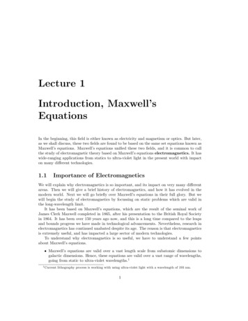
6Electromagnetic Field TheoryFigure 1.3: A brief history of electromagnetics and optics as depicted in this figure.In Figure 1.3, a brief history of electromagnetics and optics is depicted. In the beginning, it was thought that electricity and magnetism, and optics were governed by differentphysical laws. Low frequency electromagnetics was governed by the understanding of fieldsand their interaction with media. Optical phenomena were governed by ray optics, reflectionand refraction of light. But the advent of Maxwell’s equations in 1865 revealed that theycan be unified under electromagnetic theory. Then solving Maxwell’s equations becomes amathematical endeavor.The photo-electric effect [20,21], and Planck radiation law [22] point to the fact that electromagnetic energy is manifested in terms of packets of energy, indicating the corpuscularnature of light. Each unit of this energy is now known as the photon. A photon carries an energy packet equal to ω, where ω is the angular frequency of the photon and 6.626 10 34J s, the Planck constant, which is a very small constant. Hence, the higher the frequency,the easier it is to detect this packet of energy, or feel the graininess of electromagnetic energy. Eventually, in 1927 [3], quantum theory was incorporated into electromagnetics, and thequantum nature of light gives rise to the field of quantum optics. Recently, even microwavephotons have been measured [23,24]. They are difficult to detect because of the low frequencyof microwave (109 Hz) compared to optics (1015 Hz): a microwave photon carries a packet ofenergy about a million times smaller than that of optical photon.The progress in nano-fabrication [25] allows one to make optical components that aresubwavelength as the wavelength of blue light is about 450 nm. As a result, interaction oflight with nano-scale optical components requires the solution of Maxwell’s equations in itsfull glory.
Introduction, Maxwell’s Equations7In the early days of quantum theory, there were two prevailing theories of quantum interpretation. Quantum measurements were found to be random. In order to explain theprobabilistic nature of quantum measurements, Einstein posited that a random hidden variable controlled the outcome of an experiment. On the other hand, the Copenhagen schoolof interpretation led by Niels Bohr, asserted that the outcome of a quantum measurement isnot known until after a measurement [26].In 1960s, Bell’s theorem (by John Steward Bell) [27] said that an inequality should besatisfied if Einstein’s hidden variable theory was correct. Otherwise, the Copenhagen schoolof interpretation should prevail. However, experimental measurement showed that the inequality was violated, favoring the Copenhagen school of quantum interpretation [26]. Thisinterpretation says that a quantum state is in a linear superposition of states before a measurement. But after a measurement, a quantum state collapses to the state that is measured.This implies that quantum information can be hidden incognito in a quantum state. Hence,a quantum particle, such as a photon, its state is unknown until after its measurement. Inother words, quantum theory is “spooky”. This leads to growing interest in quantum information and quantum communication using photons. Quantum technology with the use ofphotons, an electromagnetic quantum particle, is a subject of growing interest. This also hasthe profound and beautiful implication that “our karma is not written on our forehead whenwe were born, our future is in our own hands!”1.2Maxwell’s Equations in Integral FormMaxwell’s equations can be presented as fundamental postulates.5 We will present them intheir integral forms, but will not belabor them until later. B · dS dE · dl dtCdH · dl dtCFaraday’s Law(1.2.1)Ampere’s Law(1.2.2)Gauss’s or Coulomb’s Law(1.2.3)Gauss’s Law(1.2.4)S D · dS Q D · dS ISSB · dS 0SThe units of the basic quantities above are given as:E: V/mD: C/m2I: AH: A/mB: W/m2Q: Cwhere V volts, A amperes, C coulombs, and W webers.5 Postulates in physics are similar to axioms in mathematics. They are assumptions that need not beproved.
81.31.3.1Electromagnetic Field TheoryStatic ElectromagneticsCoulomb’s Law (Statics)This law, developed in 1785 [28], expresses the force between two charges q1 and q2 . If thesecharges are positive, the force is repulsive and it is given byq1 q 2r̂124πεr2f1 2 (1.3.1)Figure 1.4: The force between two charges q1 and q2 . The force is repulsive if the two chargeshave the same sign.where the units are: f (force): newtonq (charge): coulombsε (permittivity): farads/meterr (distance between q1 and q2 ): mr̂12 unit vector pointing from charge 1 to charge 2r̂12 r2 r1, r2 r1 r r2 r1 (1.3.2)Since the unit vector can be defined in the above, the force between two charges can also berewritten asf1 2 1.3.2q1 q2 (r2 r1 ),4πε r2 r1 3(r1 , r2 are position vectors)(1.3.3)Electric Field E (Statics)The electric field E is defined as the force per unit charge [29]. For two charges, one of chargeq and the other one of incremental charge q, the force between the two charges, accordingto Coulomb’s law (1.3.1), isf q qr̂4πεr2(1.3.4)
Introduction, Maxwell’s Equations9where r̂ is a unit vector pointing from charge q to the incremental charge q. Then theelectric field E, which is the force per unit charge, is given byE f,4q(V/m)(1.3.5)This electric field E from a point charge q at the orgin is henceE qr̂4πεr2(1.3.6)Therefore, in general, the electric field E(r) at location r from a point charge q at r0 is givenbyE(r) q(r r0 )4πε r r0 3(1.3.7)r r0 r r0 (1.3.8)where the unit vectorr̂ Figure 1.5: Emanating E field from an electric point charge as depicted by depicted by (1.3.7)and (1.3.6).If one knows E due to a point charge, one will know E due to any charge distributionbecause any charge distribution can be decomposed into sum of point charges. For instance, if
10Electromagnetic Field Theorythere are N point charges each with amplitude qi , then by the principle of linear superposition,the total field produced by these N charges isE(r) NXqi (r ri )4πε r r i 3i 1(1.3.9)where qi %(ri ) Vi is the incremental charge at ri enclosed in the volume Vi . In thecontinuum limit, one gets E(r) V%(r0 )(r r0 )dV4πε r r0 3(1.3.10)In other words, the total field, by the principle of linear superposition, is the integral summation of the contributions from the distributed charge density %(r).
Introduction, Maxwell’s Equations1.3.311Gauss’s Law (Statics)This law is also known as Coulomb’s law as they are closely related to each other. Apparently,this simple law was first expressed by Joseph Louis Lagrange [30] and later, reexpressed byGauss in 1813 (Wikipedia).This law can be expressed as D · dS Q(1.3.11)Swhere D: electric flux density with unit C/m2 and D εE.dS: an incremental surface at the point on S given by dS n̂ where n̂ is the unit normalpointing outward away from the surface.Q: total charge enclosed by the surface S.Figure 1.6: Electric flux (courtesy of Ramo, Whinnery, and Van Duzer [31]).The left-hand side of (1.3.11) represents a surface integral over a closed surface S. Tounderstand it, one can break the surface into a sum of incremental surfaces Si , with alocal unit normal n̂i associated with it. The surface integral can then be approximated by asummation D · dS SXiDi · n̂i Si XDi · Si(1.3.12)iwhere one has defined Si n̂i Si . In the limit when Si becomes infinitesimally small,the summation becomes a surface integral.
121.3.4Electromagnetic Field TheoryDerivation of Gauss’s Law from Coulomb’s Law (Statics)From Coulomb’s law and the ensuing electric field due to a point charge, the electric flux isD εE qr̂4πr2(1.3.13)When a closed spherical surface S is drawn around the point charge q, by symmetry, theelectric flux though every point of the surface is the same. Moreover, the normal vector n̂on the surface is just r̂. Consequently, D · n̂ D · r̂ q/(4πr2 ), which is a constant on aspherical of radius r. Hence, we conclude that for a point charge q, and the pertinent electricflux D that it produces on a spherical surface, D · dS 4πr2 D · n̂ 4πr2 Dr q(1.3.14)STherefore, Gauss’s law is satisfied by a point charge.Figure 1.7: Electric flux from a point charge satisfies Gauss’s law.Even when the shape of the spherical surface S changes from a sphere to an arbitraryshape surface S, it can be shown that the total flux through S is still q. In other words, thetotal flux through sufaces S1 and S2 in Figure 1.8 are the same.This can be appreciated by taking a sliver of the angular sector as shown in Figure 1.9.Here, S1 and S2 are two incremental surfaces intercepted by this sliver of angular sector.The amount of flux passing through this incremental surface is given by dS · D n̂ · D S n̂ · r̂Dr S. Here, D r̂Dr is pointing in the r̂ direction. In S1 , n̂ is pointing in the r̂direction. But in S2 , the incremental area has been enlarged by that n̂ not aligned withD. But this enlargement is compensated by n̂ · r̂. Also, S2 has grown bigger, but the fluxat S2 has grown weaker by the ratio of (r2 /r1 )2 . Finally, the two fluxes are equal in thelimit that the sliver of angular sector becomes infinitesimally small. This proves the assertionthat the total fluxes through S1 and S2 are equal. Since the total flux from a point charge qthrough a closed surface is independent of its shape, but always equal to q, then if we have atotal charge Q which can be expressed as the sum of point charges, namely.XQ qi(1.3.15)i
Introduction, Maxwell’s Equations13Figure 1.8: Same amount of electric flux from a point charge passes through two surfaces S1and S2 .Then the total flux through a closed surface equals the total charge enclosed by it, which isthe statement of Gauss’s law or Coulomb’s law.1.4Homework ExamplesExample 1Field of a ring of charge of density %l C/m.Question: What is E along z axis? Hint: Use symmetry.Example 2Field between coaxial cylinders of unit length.Question: What is E?Hint: Use symmetry and cylindrical coordinates to express E ρ̂Eρ and appply Gauss’s law.Example 3Fields of a sphere of uniform charge density.Question: What is E?Hint: Again, use symmetry and spherical coordinates to express E r̂Er and appply Gauss’slaw.
14Electromagnetic Field TheoryFigure 1.9: When a sliver of angular sector is taken, same amount of electric flux from a pointcharge passes through two incremental surfaces S1 and S2 .Figure 1.10: Electric field of a ring of charge (courtesy of Ramo, Whinnery, and Van Duzer[31]).Figure 1.11: Figure for Example 2 for a coaxial cylinder.
Introduction, Maxwell’s EquationsFigure 1.12: Figure for Example 3 for a sphere with uniform charge density.15
16Electromagnetic Field Theory
Maxwell’s equations. Maxwell’s equations uni ed these two elds, and it is common to call the study of electromagnetic theory based on Maxwell’s equations electromagnetics. It has wide-ranging applications from statics to ultra-violet light in the present world with impact on many