WIXLIB

Since the constants may depend on the other variable y, the general solution of the PDE will beu(x, y) f (y) cos x g(y) sin x,where f and g are arbitrary functions. To check that this is indeed a solution, simply substitute theexpression back into the equation.Example 1.3. uxy 0We can think of this equation as an ODE for ux in the y variable, since (ux )y 0. Then similar tothe first example, we can integrate in y to obtainux f (x).This is an ODE for u in the x variable, which one can solve by integrating with respect to x, arrivingat at the solutionu(x, y) F (x) G(y).1.3ConclusionNotice that where the solution of an ODE contains arbitrary constants, the solution to a PDE containsarbitrary functions. In the same spirit, while an ODE of order m has m linearly independent solutions, aPDE has infinitely many (there are arbitrary functions in the solution!). These are consequences of thefact that a function of two variables contains immensely more (a whole dimension worth) of informationthan a function of only one variable.3

Problem Set 11. (#1.1.2 in [Str]) Which of the following operators are linear?(a) Lu ux xuy(b) Lu ux uuy(c) Lu ux u2y(d) Lu ux uy 1 (e) Lu 1 x2 (cos y)ux uyxy [arctan(x/y)]u2. (#1.1.3 in [Str]) For each of the following equations, state the order and whether it is nonlinear,linear inhomogeneous, or linear homogeneous; provide reasons.(a) ut uxx 1 0(b) ut uxx xu 0(c) ut uxxt uux 0(d) utt uxx x2 0(e) iut uxx u/x 0(f) ux (1 u2x ) 1/2 uy (1 u2y ) 1/2 0(g) ux ey uy 0 (h) ut uxxxx 1 u 03. Show that cos(x ct) is a solution of ut cux 0.4. (#1.1.10 in [Str]) Show that the solutions of the differential equation u000 3u00 4u 0 form avector space. Find a basis of it.5. (#1.1.11 in [Str]) Verify that u(x, y) f (x)g(y) is a solution of the PDE uuxy ux uy for all pairsof (differentiable) functions f and g of one variable.6. (#1.1.12 in [Str]) Verify by direct substitution thatun (x, y) sin nx sinh nyis a solution of uxx uyy 0 for every n 0.7. Find the general solution ofuxy ux 0.(Hint: first treat it as an ODE for ux ).4

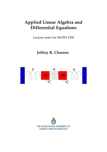
2First-order linear equationsLast time we saw how some simple PDEs can be reduced to ODEs, and subsequently solved using ODEmethods. For example, the equationux 0(2.1)has “constant in x” as its general solution, and hence u depends only on y, thus u(x, y) f (y) is thegeneral solution, with f an arbitrary function of a single variable. Today we will see that any linearfirst order PDE can be reduced to an ordinary differential equation, which will then allow as to tackleit with already familiar methods from ODEs.Let us start with a simple example. Consider the following constant coefficient PDEaux buy 0.(2.2)Here a and b are constants, such that a2 b2 6 0, i.e. at least one of the coefficients is nonzero (otherwisethis would not be a differential equation). Using the inner (scalar or dot) product in R2 , we can rewritethe left hand side of (2.2) as(a, b) · (ux , uy ) 0,or(a, b) · u 0.Denoting the vector (a, b) v, we see that the left hand side of the above equation is exactly Dv u(x, y),the directional derivative of u in the direction of the vector v. Thus the solution to (2.2) must beconstant in the direction of the vector v ai bj.yH-b, aLyΗv Ha, bLHa, bLHx, yL5Ξ5 -55x-10-5Η Hx, yL H-b, aL-5Figure 2.1: Characteristic lines bx ay c.5xΞ Hx, yL Ha, bL-5Figure 2.2: Change of coordinates.The lines parallel to the vector v have the equationbx ay c,(2.3)since the vector (b, a) is orthogonal to v, and as such is a normal vector to the lines parallel to v. Inequation (2.3) c is an arbitrary constant, which uniquely determines the particular line in this family ofparallel lines, called characteristic lines for the equation (2.2).As we saw above, u(x, y) is constant in the direction of v, hence also along the lines (2.3). The linecontaining the point (x, y) is determined by c bx ay, thus u will depend only on bx ay, that isu(x, y) f (bx ay),5(2.4)

where f is an arbitrary function. One can then check that this is the correct solution by plugging itinto the equation. Indeed,a x f (bx ay) b y f (bx ay) abf 0 (bx ay) baf 0 (bx ay) 0.The geometric viewpoint that we used to arrive at the solution is akin to solving equation (2.1) simplyby recognizing that a function with a vanishing derivative must be constant. However one can approachequation (2.2) from another perspective, by trying to reduce it to an ODE.2.1The method of characteristicsTo have an ODE, we need to eliminate one of the partial derivatives in the equation. But we know thatthe directional derivative vanishes in the direction of the vector (a, b). Let us then make a change of thecoordinate system to one that has its “x-axis” parallel to this vector, as in Figure 2. In this coordinatesystem(ξ, η) ((x, y) · (a, b), (x, y) · (b, a)) (ax by, bx ay).So the change of coordinates is ξ ax by,η bx ay.(2.5)To rewrite the equation (2.2) in this coordinates, notice that ξ η uη auξ buη , x x ξ ηuy uξ uη buξ auη . y yux uξThus,0 aux buy a(auξ buη ) b(buξ auη ) (a2 b2 )uξ .Now, since a2 b2 6 0, then, as we anticipated,uξ 0,which is an ODE. We can solve this last equation just as we did in the case of equation (2.1), arrivingat the solutionu(ξ, η) f (η).Changing back to the original coordinates gives u(x, y) f (bx ay). This is the same solution that wederived with the geometric deduction. This method of reducing the PDE to an ODE is called the methodof characteristics, and the coordinates (ξ, η) given by formulas (2.5) are called characteristic coordinates.Example 2.1. Find the solution of the equation 3ux 5uy 0 satisfying the condition u(0, y) sin y.From the above discussion we know that u will depend only on η 5x 3y, so u(x, y) f ( 5x 3y).The solution also has to satisfy the additional condition (called initial condition), which we verify byplugging in x 0 into the general solution.sin y u(0, y) f ( 3y). So f (z) sin( z3 ), and hence u(x, y) sin 5x 3y, which one can verify by substituting into the3equation and the initial condition.6

2.2General constant coefficient equationsWe can easily adapt the method of characteristics to general constant coefficient linear first-order equationsaux buy cu g(x, y).(2.6)Recall that to find the general solution of this equation it is enough to find the general solution of thehomogeneous equationaux buy cu 0,(2.7)and add to this a particular solution of the inhomogeneous equation (2.6). Notice that in the characteristic coordinates (2.5), equation (2.7) will take the form(a2 b2 )uξ cu 0,oruξ a2cu 0, b2which can be treated as an ODE in ξ. The solution to this ODE has the formuh (ξ, η) e cξa2 b2f (η),with f again being an arbitrary single-variable function. Changing the coordinates back to the original(x, y), we will obtain the general solution to the homogeneous equationuh (x, y) e c(ax by)a2 b2f (bx ay).You should verify that this indeed solves equation (2.7).To find a particular solution of (2.6), we can use the characteristic coordinates to reduce it to theinhomogeneous ODE(a2 b2 )uξ cu g(ξ, η),oruξ a2cg(ξ, η)u 2.2 ba b2Having found the solution to the homogeneous ODE, we can find the solution to this inhomogeneousequation by e.g. variation of parameters. So the particular solution will beˆcg(ξ, η) a2 b 2c 2 ξ2ξa bup eedξ.22a bThe general solution of (2.6) is then u(ξ, η) uh up ecξa2 b2 ˆcg(ξ, η) a2 b2ξedξ .f (η) a2 b 2To find the solution in terms of (x, y), one needs to first carry out the integration in ξ in the aboveformula, then replace ξ and η by their expressions in terms of x and y.Example 2.2. Find the general solution of 2ux 4uy 5u ex 3y .The characteristic change of coordinates for this equation is given by ξ 2x 4y,η 4x 2y.From these we can also find the expressions of x and y in terms of (ξ, η). In particular notice thatx 3y ξ η. In the characteristic coordinates the equation reduces to220uξ 5u e7ξ η2.

The general solution of the homogeneous equation associated with the above equation is1uh e 4 ξ f (η),and the particular solution will beup e 14 ξˆξ η11e 2 1ξ1 η 31 1e 4 dξ e 4 ξ · e 2 e 4 ξ e 4 ξ · e 4 (3ξ 2η) .201515Adding these two will give the general solution to the inhomogeneous equation 1 1 (3ξ 2η) 41 ξu(ξ, η) ef (η) e 4.15Finally, substituting the expressions for ξ and η in terms of (x, y), we will obtain the solution 1 1 (2x 16y) 41 (2x 4y)f (4x 2y) e 4.u(x, y) e15You should check that this indeed solves the differential equation.2.3Variable coefficient equationsThe method of characteristics can be generalized to variable coefficient first-order linear PDEs as well,albeit the change of variables may no longer be orthogonal. The general variable coefficient linearfirst-order equations isa(x, y)ux b(x, y)uy c(x, y)u d(x, y).(2.8)Let us first consider the following simple particular caseux yuy 0.(2.9)Using our geometric intuition from the constant coefficient equations, we see that the directional derivative of u in the direction of the vector v (1, y) is constant. Notice that the vector v itself is no longerconstant, and varies with y. The curves that have v as their tangent vector have slope y1 , and thus satisfyydy .dx1We can solve this equation as an ODE, and obtain the general solutiony Cex ,ore x y C.(2.10)As in the case of the constant coefficients, the solution to the equation (2.9) will be constant along thesecurves, called characteristic curves. This family of non-intersecting curves fills the entire coordinateplane, and the curve containing the point (x, y) is uniquely determined by C e x y, which implies thatthe general solution to (2.9) isu(x, y) f (C) f (e x y).As always, we can check this by substitution.ux yuy f 0 (e x y)e x y yf 0 (e x y)e x 0.Let us now try to generalize the method of characteristics to the equationa(x, y)ux b(x, y)uy 0.8(2.11)

The idea is again to introduce new coordinates (ξ, η), which will reduce (2.11) to an ODE. Suppose ξ ξ(x, y),(2.12)η η(x, y)gives such a change of variables. To rewrite the equation in this coordinates, we computeux uξ ξx uη ηx ,uy uξ ξy uη ηy ,and substitute these into equation (2.11) to get(aξx bξy )uξ (aηx bηy )uη 0.Since we would like this to give us an ODE, say in ξ, we require the coefficient of uη to be zero,aηx bηy 0.Without loss of generality, we may assume that a 6 0 (locally). Notice that for curves y(x) that havedy ab we havethe slope dxdbdyη(x, y(x)) ηx ηy ηx ηy 0.dxdxaSo the characteristic curves, just as before, are given bybdy .dxa(2.13)The general solution to this ODE will be η(x, y) C, with ηy 6 0 (otherwise ηx 0 as well, and thiswill not be a solution). This is how we find the new variable η, for which our PDE reduces to an ODE.We choose ξ(x, y) x as the other variable. For this change of coordinates the Jacobian determinant isJ (ξ, η)ξ ξ x y ηy 6 0.ηx ηy (x, y)Thus, (2.12) constitutes a non-degenerate change of coordinates. In the new variables equation (2.11)reduces toa(ξ, η)uξ 0, hence uξ 0,which has the solutionu f (η).The general variable coefficient equation (2.8) in these coordinates will reduce toa(ξ, η)uξ c(ξ, η)u d(ξ, η),which is called the canonical form of equation (2.8). This equation, as in previous cases, can be solvedby standard ODE methods.Example 2.3. Find the general solution of the equationxux yuy y 2 u y 2 ,x, y 6 0.dyCondition (2.13) in this case is dx xy . This is a separable ODE, which can be solved to obtain thegeneral solution xy C. Thus, our change of coordinates will be ξ x,η xy.9

In these coordinates the equation takes the formξuξ η2η2u ,ξ2ξ2Using the integrating factor eη2ξ3or uξ dξ e η22ξ2η2η2u .ξ3ξ3,the above equation can be written as 222 η2 η ηe 2ξ u e 2ξ2 3 .ξξIntegrating both sides in ξ, we arrive at eη22ξ2ˆu e η22ξ22η2 η22ξ f (η).dξ eξ3Thus, the general solution will be given by 2η2η2 η22u(ξ, η) e 2ξ f (η) e 2ξ e 2ξ2 f (η) 1.Finally, substituting the expressions of ξ and η in terms of (x, y) into the solution, we obtainy2u(x, y) f (xy)e 2 1.One should again check by substitution that this is indeed a solution to the PDE.2.4ConclusionThe method of characteristics is a powerful method that allows one to reduce any first-order linear PDEto an ODE, which can be subsequently solved using ODE techniques. We will see in later lectures thata subclass of second order PDEs – second order hyperbolic equations can be also treated with a similarcharacteristic method.10

33.1Method of characteristics revisitedTransport equationA particular example of a first order constant coefficient linear equation is the transport, or advectionequation ut cux 0, which describes motions with constant speed. One way to derive the transportequation is to consider the dynamics of the concentration of a pollutant in a stream of water flowingthrough a thin tube at a constant speed c.Let u(t, x) denote the concentration of the pollutant in gr/cm (unit mass per unit length) at time t.The amount of pollutant in the interval [a, b] at time t is thenˆbu(x, t) dx.aDue to conservation of mass, the above quantity must be equal to the amount of the pollutant aftersome time h. After the time h, the pollutant would have flown to the interval [a ch, b ch], thus theconservation of mass givesˆˆbb chu(x, t) dx au(x, t h) dx.a chTo derive the dynamics of the concentration u(x, t), differentiate the above identity with respect to b togetu(b, t) u(b ch, t h).Notice that this equation asserts that the concentration at the point b at time t is equal to the concentration at the point b ch at time t h, which is to be expected, due to the fact that the watercontaining the pollutant particles flows with a constant speed. Since b is arbitrary in the last equation,we replace it with x. Now differentiate both sides of the equation with respect to h, and set h equal tozero to obtain the following differential equation for u(x, t).0 cux (x, t) ut (x, t),orut cux 0.(3.1)Since equation (3.1) is a first order linear PDE with constant coefficients, we can solve it by themethod of characteristics. First, we rewrite the equation as(1, c) · u 0,which implies that the slope of the characteristic lines is given bydxc .dt1Integrating this equation, one arrives at the equation for the characteristic linesx ct x(0),(3.2)where x(0) is the coordinate of the point at which the characteristic line intersects the x-axis. Thesolution to the PDE (3.1) can then be written asu(t, x) f (x ct)for any arbitrary single-variable function f .11(3.3)

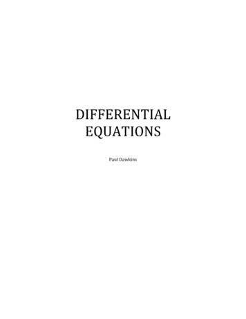
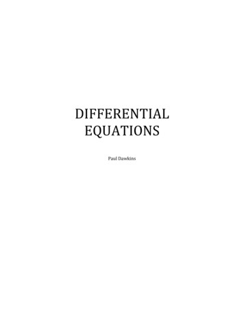
Let us now consider a particular initial condition for u(t, x) x0 x 1,u(0, x) 0otherwise.(3.4)According to (3.3), u(0, x) f (x), which determines the function f . Having found the function from theinitial condition, we can now evaluate the solution u(t, x) of the transport equation from (3.3). Indeed x ct0 x ct 1u(t, x) f (x ct) 0otherwiseNoticing that the inequalities 0 x ct 1 imply that x is in-between ct and ct 1, we can rewritethe above solution as x ctct x ct 1,u(t, x) 0otherwise,which is exactly the initial function u(0, x), given by (3.4), moved to the right along the x-axis by ctunits. Thus, the initial data u(0, x) travels from left to right with constant speed c.We can alternatively understand the dynamics by looking at the characteristic lines in the xt coordinate plane. From (3.2), we can rewrite the characteristics as1t (x x(0)).cAlong these characteristics the solution remains constant, and one can obtain the value of the solutionat any point (t, x) by tracing it back to the x-axis:u(t, x) u(t t, x ct) u(0, x(0)).tuut 0t 3xxFigure 3.2: The graph of u(t, x) colored with respect to time t.Figure 3.1: u(t, x) at two different times t.Figure 1 gives the graphs of u(t, x) at two different times, while Figure 3.1 gives the three dimensionalgraph of u(t, x) as a function of two variables.3.2Quasilinear equationsWe next look at a simple nonlinear equation, for which the method of characteristics can be applied aswell. The general first order quasilinear equation has the following forma(x, y, u)ux b(x, y, u)uy g(x, y, u).12

We can see that the highest order derivatives, in this case the first order derivatives, enter the equationlinearly, although the coefficients depend on the unknown u. A very particular example of first orderquasilinear equations is the inviscid Burger’s equationut uux 0.(3.5)As before, we can rewrite this equation in the form of a dot product, which is a vanishing condition fora certain directional derivative(1, u) · (ut , ux ) 0,or(1, u) · u 0.This shows that the tangent vector of the characteristic curves, v (1, u), depends on the unknownfunction u.3.3RarefactionLet as now look at a particular initial condition, and try to construct solutions along the characteristiccurves. Suppose 1if x 0,u(0, x) (3.6)2if x 0.The slope of the characteristic curves satisfiesdx u(t, x(t)) u(0, x(0)).dtHere we used the fact that the directional derivative of the solution vanishes in the direction of thetangent vector of the characteristi

PARTIAL DIFFERENTIAL EQUATIONS Math 124A { Fall 2010 « Viktor Grigoryan grigoryan@math.ucsb.edu Department of Mathematics University of California, Santa Barbara These lecture notes arose from the course \Partial Di erential Equations" { Math 124A taught by the author in the Department of M