Transcription
Seismic Hazard Curves andUniform Hazard Response Spectrafor the United Statesby A. D. Frankel and E. V. LeyendeckerA User Guide to AccompanyOpen-File Report 01-4362001This report is preliminary and has not been reviewed for conformity with U.S. Geological Surveyeditorial standards or with the North American Stratigraphic Code. Any use of trade firm or productnames is for descriptive purposes only and does not imply endorsement by the U.S. Government.U.S. DEPARTMENT OF THE INTERIORGale A. Norton, SecretaryU.S. GEOLOGICAL SURVEYCharles G. Groat, Director
Seismic Hazard Curves and Uniform Hazard Response Spectrafor the United StatesA User Guide to Accompany Open-File Report 01-436A. D. Frankel1 and E. V. Leyendecker2ABSTRACTThe U.S. Geological Survey (USGS) recently completed newprobabilistic seismic hazard maps for the United States. The hazard mapsform the basis of the probabilistic component of the design maps used inthe 2000 International Building Code (International Code Council,2000a), 2000 International Residential Code (International Code Council,2000a), 1997 NEHRP Recommended Provisions for Seismic Regulationsfor New Buildings (Building Seismic Safety Council, 1997), and 1997NEHRP Guidelines for the Seismic Rehabilitation of Buildings (AppliedTechnology Council, 1997).The probabilistic maps depict peakhorizontal ground acceleration and spectral response at 0.2, 0.3, and 1.0sec periods, with 10%, 5%, and 2% probabilities of exceedance in 50years, corresponding to return times of about 500, 1000, and 2500 years,respectively.This report is a user guide for a CD-ROM that has been prepared toallow the determination of probabilistic map values by latitude-longitudeor zip code. The CD includes additional spectral accelerations at 0.1, 0.5,and 2.0 sec for the 48 conterminous states. The CD also contains hazardcurve data that were used to prepare the maps. Hazard curves may also bedetermined by latitude-longitude or zip code.1 Geophysicist, U.S. Geological Survey, MS 966, Box 25046, DFC, Denver, CO, 802252 Research Civil Engineer, U.S. Geological Survey, MS 966, Box 25046, DFC, Denver, CO, 802251
INTRODUCTIONIn June 1996 the USGS completed new national seismic hazard maps for the conterminousUnited States. These maps were placed on the Internet (http://geohazards.cr.usgs.gov/eq/) andsubsequently published as large format maps. There are two sets of maps available for the 48conterminous states. The first set covers all 48 states (Frankel et al., 1997 a), the second set isfor region A of Figure A (Frankel et al.,1997 b). This regional set of maps coversCalifornia, Nevada, and portions ofwestern Utah and Arizona.Each set ofthese hazard maps includes maps of peakhorizontal ground acceleration andspectral response at 0.2, 0.3, and 1.0 secperiods, for 10%, 5%, and 2%probabilities of exceedance in 50 years.These probabilities of exceedancecorrespond to return times of about 500,1000, and 2500 years, respectively. Newhazard maps for Alaska (Wesson et al., Figure A. Regional map A. The regional map includes1999 a, b) and Hawaii (Klein et al., 2000)California, Nevada, and western portions of Utah andhave recently been completed. Each set ofArizona.these hazard maps includes maps of peakhorizontal ground acceleration and spectral response at 0.2, 0.3, and 1.0 sec periods, for 10% and2% probabilities of exceedance in 50 years, corresponding to return times of about 500 and 2500years, respectively. The 5% probability of exceedance maps were omitted for Alaska andHawaii after it was found that the demand for these maps was limited. The methodology usedfor preparation of the maps is documented in Frankel et al (1996), Wesson et al (1999), andKlein et al (draft, 1998). Copies of these reports are included with this CD-ROM. A summarypaper describing the hazard maps is available in a special edition of Spectra (Frankel et al.,2000).The mapping project was part of “Project 97" with the Building Seismic Safety Council(BSSC) to produce seismic design maps for the 1997 NEHRP Recommended Provisions forSeismic Regulations for New Buildings (hereafter referred to as NEHRP Provisions). The designmaps in the 1997 NEHRP Provisions are a combination of probabilistic seismic hazard maps formost of the U.S. and deterministic hazard maps near specific faults in California, Oregon,Washington, Alaska, and Hawaii. The design maps originally prepared for the NEHRPProvisions have also been adopted for use in the 1997 NEHRP Guidelines for the SeismicRehabilitation of Buildings (ATC, 1997), International Building Code (ICC, 2000), and theInternational Residential Code (ICC, 2000). A summary paper describing the design maps isalso available in the special edition of Spectra (Leyendecker et al., 2000) mentioned above.2
The hazard maps serve a number of purposes, e.g. site studies, structural design, earthquakeloss studies, etc. Although simple in approach, it can be cumbersome to work with multiplemaps. In order to simplify use of the ground motion maps the CD-ROM described in this reportwas prepared. The original intent of the CD-ROM was to enable a user to determine map valuesfor a site by zip code or latitude-longitude. However, it was soon discovered that thepossibilities were much broader.The CD-ROM provides three basic sets of information to the user (1) map files, (2)hazardcurve data, and (3) spectral response acceleration data. The hazard curve and spectral responseacceleration data may be obtained in tabular or graphical form by specifying a site location bylatitude-longitude or zip code. The CD also contains the map files for the four map setsdescribed earlier.The data base used with the CD-ROM is the same as that used to prepare the maps. Theparameters used to prepare each map were calculated on a grid for the areas to be mapped, themaps were then constructed by contouring the “gridded data”. The grid spacing was 0.1 deg forthe 48 conterminous states (except Region A was also calculated at a grid of 0.05 deg) andAlaska. Hawaii maps were constructed using calculations at a grid spacing of 0.02 deg.SOFTWARE AND USER GUIDEA program, Probabilistic Hazard 3.10, was written to retrieve the various data on the CD.The program was written in Visual Basic 6.0 to operate on a PC with a Windows 95 or lateroperating system. It self installs and uses the usual mouse and point and click approach tooperate. The program allows the user to calculate both a hazard curve and a uniform hazardresponse spectrum for a specified site. The program also opens the map files for viewing. Someof the program features are described below. More detail is provided in Figures 1 through 16with the detailed information in the figure captions. Table 1 shows the general information forinstalling and operating the software.HAZARD MAPSAll of the maps in the four map sets of the United States described in the Introduction areincluded in the subdirectory “GM96-MAPS” on the CD-ROM, in pdf format. The program,Probabilistic Hazard 3.10, is used to view the various maps by selecting from a list of the maps.Once a map is selected, the program opens Acrobat Reader (copyright Adobe) with the map.The program uses Acrobat Reader to view and manipulate the maps, such as zooming andprinting. The maps may also be viewed using Acrobat Reader independently of ProbabilisticHazard.3
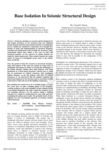
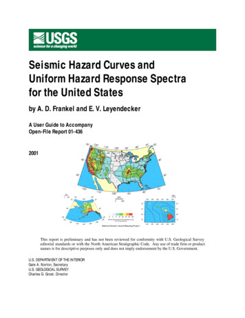
HAZARD CURVESA sample hazard curve is shown in Figure B. A hazard curve, as calculated on the CD, is aplot of the annual frequency of exceedance (FEX) versus peak ground acceleration or one of thespectral accelerations. The hazard curve for peak groundacceleration shown in Figure B was calculated for aspecific site, located by latitude-longitude, by interpolatingdata at the surrounding four grid points. Data used toprepare the graph are also tabulated along with the plot.The program allows the user to print the data in hard copyor save it in an ASCII comma-delimited file. Data saved inthis type of file can be imported into a large variety ofsoftware, such as a spreadsheet program, for additionalprocessing as specified by the user.The maps were prepared by computing such hazardcurves at each grid point within the mapping area. FEXvalues of 0.0021, 0.00103, and 0.000404 correspond to Figure B. Sample seismic hazardprobabilities of exceedance of 10% in 50 years, 5% in 50curve for peak groundyears, and 2% in 50 years respectively. The hazard curveacceleration Data points areshown as solid circles.was then used to determine the acceleration valuecorresponding to each of these three FEX values and storedin a data base. This procedure was repeated at each grid point, for each ground motionparameter. This process created the “gridded data” referred to above that was used to prepare themaps.RESPONSE SPECTRAAlthough maps were not made, hazard curves were also developed for spectral accelerationsat 0.1, 0.5, and 2.0 sec for the 48 conterminous states in addition to hazard curves for peakground acceleration and spectral accelerations at 0.2, 0.3,and 1.0 sec. These additional values were not computed forHawaii or Alaska because appropriate ground motionattenuation equations were not available for these periodsfor these geographical regions. The peak groundacceleration and spectral accelerations corresponding toeach of the three standard probabilities were used to createa data base for response spectra for the three probabilitylevels at each grid point. A sample response spectrum for a2% probability of exceedance in 50 years is shown inFigure C. Response spectra can also be computed for 5% Figure C. Sample uniform hazardresponse spectrum for 2% PE inand 10% probability of exceedance in 50 years. As was the50 years.case for hazard curves, data used to prepare the graph arealso tabulated. The program allows the user to print thedata in hard copy or save it in an ASCII comma-delimited file. The current version of thesoftware does not allow saving the graph in a separate file.4
CONCLUDING REMARKSThe CD-ROM has been developed to simplify obtaining mapped ground motions and hazard.The CD is intended to be as user friendly as possible and to quickly give the user the data neededfor various purposes, such as design or site studies. The intent of USGS is to simplify andreduce the time required to obtain data from a large set of maps.It should be noted that the values obtained from the CD are the same as the values for theprobabilistic component of the design maps in NEHRP Provisions and the other designdocuments which have incorporated the design maps. However, the probabilistic values differfrom the deterministic component of the design maps.As previously indicated, the user guide is developed as a series of figures numbered Figure 1through 16 following this text. Each figure is a screen copy obtained while running the program.The caption for each figure contains extensive text so the user does not have to go back and forthbetween text and figure. The figures go through an example for calculating a response spectrumin some detail, followed by an example for calculating a hazard curve. Use of the map viewercapability is also illustrated. It is suggested the user run the software using the information inthe figures as a tutorial to gain experience in using the software.Comments and suggestions are welcome and may be sent to the individuals named below:E. V. Leyendeckeremail - leyendecker@usgs.govPhone 303-273-8565FAX 303-273-8600U. S. Geological SurveyP. O. Box 25046, MS 966Denver, CO 80225A. D. Frankelemail - afrankel@usgs.govPhone 303-273-8556FAX 303-273-8600U. S. Geological SurveyP. O. Box 25046, MS 966Denver, CO 80225ACKNOWLEDGMENTSThe authors received comments and suggestions from many individuals while preparing thisversion of the CDROM. These suggestions are gratefully acknowledged. Two individuals,Richard D. McConnell and Michael Valley, were particularly thorough and offered many wellconsidered suggestions, most of which were incorporated into this version of the software on theCD-ROM.5
REFERENCESApplied Technology Council, 1997, NEHRP Guidelines for the Seismic Rehabilitation of Buildings,FEMA 273, Washington, D. C.Building Seismic Safety Council, 1998, NEHRP Recommended Provisions for Seismic Regulations forNew Buildings and Other Structures, FEMA 302, Part 1- Provisions, FEMA 303, Part 2 Commentary, Washington, D.C.Frankel A.D., Mueller, C.S., Barnhard, T.P., Perkins, D.M., Leyendecker, E.V., Dickman, N.C., Hanson,S.L., and Hopper, M.G., 1996, National Seismic Hazard Maps, June 1996: Documentation, U.S.Geological Survey, Open-file Report 96-532.Frankel A.D., Mueller, C.S., Barnhard, T.P., Perkins, D.M., Leyendecker, E.V., Dickman, N.C., Hanson,S.L., and Hopper, M.G., 1997a, Seismic - Hazard Maps for the Conterminous United States: U.S.Geological Survey, Open-file Report 97-130, 12 sheets, scale 1:7,000,000.Frankel A.D., Mueller, C.S., Barnhard, T.P., Perkins, D.M., Leyendecker, E.V., Dickman, N.C., Hanson,S.L., and Hopper, M.G., 1997b, Seismic-Hazard Maps for the California, Nevada and WesternArizona/Utah: U.S. Geological Survey, Open-file Report 97-130, 12 sheets, scale 1:2,000,000.Frankel, A.D., Mueller, C.S., Barnhard, T.P., Leyendecker, E.V., Wesson, R.L., Harmsen, S.C., Klein,F.W., Perkins, D.M., Dickman, N.C., Hanson, S.L., and Hopper, M.G., 2000, AUSGS NationalSeismic Hazard Maps”, Spectra, Earthquake Engineering Research Institute, Oakland, CA.International Code Council, Inc., 2000a, International Building Code, Building Officials and CodeAdministrators International, Inc., Country Club Hills, IL; International Conference of BuildingOfficials, Whittier, CA; and Southern Building Code Congress International, Inc., Birmingham, AL.International Code Council, Inc., 2000b, International Residential Code, Building Officials and CodeAdministrators International, Inc., Country Club Hills, IL; International Conference of BuildingOfficials, Whittier, C. A., and Southern Building Code Congress International, Inc., Birmingham, AL.Klein, F.W., Frankel, A.D., Mueller, C.S., Wesson, R.L., and Okubo, P.G., 1998 (draft), Documentationfor Seismic Hazard Maps for the State of Hawaii (draft), available in draft form.Klein, F.W., Frankel, A.D., Mueller, C.S., Wesson, R.L., and Okubo, P.G., 2000, Seismic - Hazard Mapsfor Hawaii: U.S. Geological Survey, Geologic Investigation Series Maps I-2724, 2 sheets.Leyendecker, E. V., Hunt, R. J., Frankel, A. D., and Rukstales, K. S., 2000. “Development of MaximumConsidered Earthquake Ground Motion Maps”, Spectra, Earthquake Engineering Research Institute,Spectra , Oakland, CA.Wesson, R.L., Frankel A.D., Mueller, C.S., and Harmsen, S.C., 1999, Probabilistic Seismic Hazard Mapsof Alaska, U.S. Geological Survey, Open-file Report 99-36.Wesson, R.L., Frankel A.D., Mueller, C.S., and Harmsen, S.C., 1999, Seismic - Hazard Maps for Alaska:U.S. Geological Survey, Geologic Investigation Maps I-2679, 2 sheets.6
Table 1.General Instructions for theProgramInstallationClick on Start.Run Setup.exe in the root directory on the CDROM and followthe instructions.You may be requested to update selected files. This is required.The program will be installed in the directory ProbabilisticHazard 3.10 with an executable file named ProbabilisticHazard 3.10.exe.System RequirementsA PC (or compatible) with Windows 95, Windows 98, orWindows NT.Pentium Processor with 32 MB of RAM, 200 MHZrecommended.A minimum screen resolution of at least 800 x 600.A hard drive with 30 MB available for installing the software.OperationClick on Start.Click on Programs.Select Probabilistic Hazard 3.10 from the Programs list or placean icon on the Desktop.FilesRandom Access Data files are in the directory GM96-Data on theCD.PDF Map files are in the directory GM96-Maps on the CD.Adobe Acrobat is required to view the maps. Acrobat Readerversion 4 is included on the CD. Version 4 is recommendedfor maximum benefit in viewing and printing the PDF mapfiles.7
Figure 1.Seismic Hazard Curves and Uniform Hazard Response Spectra. The opening screen containscontrols for obtaining seismic data for both probabilistic hazard curves and response spectra.Typically a control may be accessed in three ways - (1) using the Mouse to place the cursorover the control and pressing the left Mouse button, (2) using the Tab key to cycle throughthe controls and pressing the Enter key, or (3) holding down the Alt key and pressing theunderlined character on the key. Many users will find methods (1) and (3) a convenient wayto move rapidly between controls and screens. Use whatever method or combination ofmethods is most convenient. Selecting the control labeled Hazard Curves and ResponseSpectra for the United States will open the screen shown in Figure 2. Figure 2 will be usedto illustrate most of the controls and screens. The Exit Program control closes the program.8
Figure 2.Uniform Hazard Spectra and Seismic Hazard Curves. Selecting the control discussed inFigure 1 opened the screen shown in this figure. The contents of the screen are accessedsequentially. Portions that can not be accessed are grayed out. In general, the user is guidedthrough the program by the use of titles in red and controls with titles in black. This is a clueas to what control or option should be used next. At the point shown in the figure, the usermay use the option for entering a name and date or proceed directly to the Open FileSelection Menu control. Although not required, this option is a convenient way to include aname or project description in the output. The option is followed by selecting the Open FileSelection Menu control. Throughout the program, “tool tips” (notes with a yellowbackground that explain the meaning or use of a control) will appear if the cursor is heldover a control or option. Note that in this screen the user may return to the screen in Figure 1by selecting the Opening Menu control. The Exit Program control closes the program.9
Figure 3.Optional Name and Date Entry. The name and date option have been selected. Both will beincluded with the output calculations. If only one is selected, then only the one will beincluded. The date and time are the computer time. In this case a project description hasbeen entered instead of a name. The name indicates that the following series of screens willbe an example of determining a response spectrum.In order to proceed, the user must select the Open File Selection Menu control.10
Figure 4.Select File Locations. The data files and the map files may be accessed on the CD ROM orfrom a location on a hard drive or any other drive with sufficient space to hold them. In thecase shown the directories containing the files have been copied to the C: drive. Location ona hard drive will usually allow faster access time than using the files located on the CD ROM.If the files are relocated, the names of the directories containing the files should be the sameas those on the CD ROM, although this is not necessary. The user may also manually enterthe location of files in the text boxes. An error message will appear if an incorrect drive isselected. The software checks to be sure that each data file and map file is in the designateddirectory. All files must be present before proceeding.Once the location of the files has been entered, that location is remembered for future runs ofthe software. However, if the files are moved, a new path must be entered. Press OK toreturn to the main menu. As long as the correct file locations are shown in the text boxes, allthe user has to do is click on OK, regardless of what is shown elsewhere on the screen.11
Figure 5.Select Geographic Region. Geographic Regions may be selected by clicking on the text.The selected region is highlighted in blue. Site locations for the conterminous 48 states,Alaska, and Hawaii may be specified by latitude-longitude or zip code as shown in the SelectSite Location frame. The so-called “radio buttons” may be used to select either method oflocating a site. The buttons are shown in white and their descriptions are shown in blue. Thecontrol View Maps allows the user to access the maps used in the various design procedures.Notice that a list of parameters that now appears in the list box in the frame to Calculate UHS orHazard Curve. These parameters may not be selected until the method of specifying a site hasbeen specified.12
Figure 6.Select Site Location. Site locations may be specified by either latitude-longitude or zip code.The latitude-longitude option has been selected in this screen. Notice that the latitudelongitude range is shown adjacent tothe text box for entering values. The range changesaccording to the geographic region selected. If the site is specified by zip code, the centralvalues of the zip code are computed and shown in the text boxes. It is important to be awarethat when the zip code option is selected, the value is determined at the central values shown.They are not maximum or minimum values for the zip code. In some areas, such as coastalCalifornia, there may be significant variation within a zip code. The user may get an idea ofthe variation by entering different latitude-longitude pairs near the central values or looking atcontours on the probabilistic hazard maps. The maps, included on the CDROM, arediscussed later.The control Clear Selections clears the data related to specifying a site.13
Figure 7.Calculate Spectrum. The spectral values for the U.H.S. for 2% PE in 50 years (highlighted inblue) were calculated by pressing the Calculate Spectrum control. Notice the optional nameand date are shown with the output. The latitude and longitude used to calculate the valuesare also shown so there is a record of the input along with the output. The values arecalculated by interpolation using the four surrounding grid points. These grid points are inthe data files in the directory GM96-Data on the CD. Data are located at different gridspacing for different regions. In the case shown the grid spacing is 0.05 degree. In thecentral and eastern United States the spacing is 0.1 degree. This latter spacing would not beadequate for a region such as the southwestern United States, particularly California, wherethere are many faults. The Alaska grid spacing is 0.1 degree and the Hawaii grid spacing is0.02 degree.There are four additional controls shown below the output box that are now active. These aredescribed below:Clear Output clears the contents of the output box.Clear All combines Clear Selections and Clear Output.Save To File saves the contents of the output box to an ASCII comma-delimited file.Print sends the contents of the output box to a printer.14
Figure 8.Response Spectrum Plot. A spectrum based on the data in Figure 7 is shown in the plot. Thespectral values are shown as solid blue circles. The values used to prepare the plot are shownin the adjacent list box. These are the same as those in the output box shown in Figure 7.The plot includes data, site location, soil factors, and type of ground motion (2% in 50 yearsin this case). The plot and its data points may be printed by selecting Print Spectrum. In thecurrent version of the software, the figure may not be saved as a file.15
Figure 9.Calculate Spectrum for Alaska. In this example, the spectral values were calculated for alocation in Alaska for a U.H.S. for 10% PE in 50 years (highlighted in blue). It may beobserved that the calculations are cumulative with the calculations in Figure 7. Calculationswill not be cumulative if the Clear Output control is pressed between calculations. It mayalso be observed that there are not as many spectral values for the site in Alaska as there werein the lower 48 states. Locations in Alaska and Hawaii do not have spectral values calculatedfor periods of 0.1, 0.5, and 2.0 sec because there were not appropriate attenuation functionsfor these periods in these two geographical regions.16
Figure 10. Response Spectrum Plot for Alaska.The data in Figure 9 are shown in the plot. Thespectral values are shown as solid red circles. The main difference between the content ofthis plot and the one shown in Figure 8 (other than the different location) is that dashed linesare drawn through the data. The lines are shown dashed to illustrate the general trends of thedata although, due to the lack of additional spectral values, it is considered more appropriateto leave interpretation of the intermediate values to the judgment of the professional using thedata. These same remarks apply to spectral plots for sites in Hawaii.17
Figure 11. Calculate Hazard Curve. The hazard curve for peak ground acceleration (highlighted inblue) was calculated by pressing the Calculate Hazard Curve control. Notice that the namesof the “Calculate” and “View” controls have changed from the names in Figure 9. Thesecontrols depend on whether the selected parameter is a U.H.S. or a Hazard Curve. In thisexample, a zip code was used to specify the site. The latitude and longitude are the centralvalues for the zip code. These values are in the program data base for the zip code. Aspreviously noted, it is important to be aware that when the zip code option is selected, theground motion parameters are determined at the central values shown. They are notmaximum or minimum values for the zip code. In some areas, such as coastal California,there may be significant variation within a zip code. The zip code and the latitude-longitudeused to calculate the values are also shown in the output so there is a record of the input alongwith the output. The hazard curve values are interpolated to the site based on the surroundingfour grid points. This is the same procedure used to interpolate the spectral values.18
Figure 12. Hazard Curve Plot. A hazard curve based on the data in Figure 11 is shown in the plot. Thedata are shown as solid blue circles. The values used to prepare the plot are shown in theadjacent list box. These are the same as those in the output box shown in Figure 11. The plotincludes data, site location, site condition, and type of hazard curve (PGA in this case). Theplot and its data points may be printed by selecting Print Hazard Curve. The figure may notbe saved as a separate file.FEX is the annual frequency of exceedance. The user is cautioned that values smaller than10-4 should be used with carefully. This precaution is because such values are usuallyassociated with critical structures. Such structures frequently warrant special site studyconsiderations that may or may not have been incorporated in the national maps. FEX valuesof 0.0021, 0.00103, and 0.000404 correspond to probabilities of exceedance of 10% in 50years, 5% in 50 years, and 2% in 50 years respectively.19
Figure 13. Select Map File. The maps may be viewed at any time after the file locations have beenspecified. Clicking on the View Maps control shown Figure 5, 6, or 7 opens the menushown. Click on a map to enable the View Map button. Click the View Map control to loadthe map. The map sets include the probabalistic maps for the 48 conterminous states, thesouthwestern U.S., Alaska, and Hawaii. The map selected above is shown in Figure 14.Selecting the control Notes for First Time Users opens the screen in Figure 15. Selecting thecontrol Select New Path for Acrobat Reader opens the screen shown in Figure 16.20
21Figure 14. Acrobat Reader. The program automatically opens Acrobat Reader and loads the map file. The map shown isdifficult to read because it is a reduction from the original size of about 24" x 36". It becomes easier to read when themagnification tool is used to zoom into an area. After zooming in, the graphics select tool can be used to selectdetailed portions of the map for printing. Use the Close Map control to close the reader.
Figure 15. Adobe Acrobat Reader Installation. Acrobat Reader 4.0 is necessary to view and print themaps or portions of the maps. Earlier releases of the Reader give unpredictable results in lineweights and do not allow printing selected portions of the maps.Special instructions must be followed to allow automatic loading of map files. This screenwith the installation instructions is accessed by selecting the control Notes for First TimeUsers in Figure 13.22
Figure 16. User-Specified Acrobat Reader Location. This screen is accessed by selecting the controlSelect New Path for Acrobat Reader shown in figure 13. It is not necessary to enter a path ifthe default path is the correct installation location. In the selections shown above, the defaultpath has been selected. Notice that the default path is shown as a guide to the user to selectanother path for the Reader. The version of the Reader included with this CDROM willautomatically be installed in this location.23
The program was written in Visual Basic 6.0 to operate on a PC with a Windows 95 or later operating system. It self installs and uses the usual mouse and point and click approach to operate. The program allows the user to calculate both a hazard curve and a uniform hazard response spectrum for a specified site.