Transcription
Cambridge University Press978-0-521-19910-0 - Practical Seismic Data AnalysisHua-Wei ZhouExcerptMore information1Introduction to seismic data and processingChapter contents1.1Seismic data and their acquisition, processing, and interpretation1.2Sampled time series, sampling rate, and aliasing1.3Seismic amplitude and gain control1.4Phase and Hilbert transforms1.5Data format and quality control (QC)1.6SummaryFurther readingThe discipline of subsurface seismic imaging, or mapping the subsurface using seismicwaves, takes a remote sensing approach to probe the Earth’s interior. It measuresground motion along the surface and in wellbores, then puts the recorded data througha series of data processing steps to produce seismic images of the Earth’s interior interms of variations in seismic velocity and density. The ground movements recorded byseismic sensors (such as geophones and seismometers onshore, or hydrophones andocean bottom seismometers offshore) contain information on the media’s response tothe seismic wave energy that traverses them. Hence the first topic of this chapter is onseismic data and their acquisition, processing, and interpretation processes. Becausenearly all modern seismic data are in digital form in order to be stored and analyzedin computers, we need to learn several important concepts about sampled time seriessuch as sampling rate and aliasing; the latter is an artifact due to under-sampling. Inexploration seismology, many useful and quantifiable properties of seismic data arecalled seismic attributes. Two of the most common seismic attributes are the amplitudeand phase of seismic wiggles. They are introduced here together with relevant processingissues such as gain control, phase properties of wavelets, and the Hilbert transform, in this web service Cambridge University Presswww.cambridge.org
Cambridge University Press978-0-521-19910-0 - Practical Seismic Data AnalysisHua-Wei ZhouExcerptMore information2Practical Seismic Data Analysiswhich enables many time-domain seismic attributes to be extracted. To process realseismic data, we also need to know the basic issues of data formats, the rules of storingseismic data in computers. To assure that the data processing works, we need toconduct many quality control checks. These two topics are discussed together becausein practice some simple quality control measures need to be applied at the beginningstage of a processing project.A newcomer to the field of seismic data processing needs to know the fundamentalprinciples as well as common technical terms in their new field. In this book, phrasesin boldface denote where special terms or concepts are defined or discussed. Tocomprehend each new term or concept, a reader should try to define the term in hisor her own words. The subject of seismic data processing often uses mathematicalformulas to quantify the physical concepts and logic behind the processing sequences.The reader should try to learn the relevant mathematics as much as possible, and, atthe very least, try to understand the physical basis and potential applications for eachformula. Although it is impossible for this book to endorse particular seismic processingsoftware, readers are encouraged to use any commercially or openly accessible seismicprocessing software while learning seismic data processing procedures and exercises.An advanced learner should try to write computer code for important processing stepsto allow an in-depth comprehension of the practical issues and limitations.1.1Seismic data and their acquisition, processing, and interpretation.As a newcomer, you first want to know the big picture: the current and future objectivesand practices of seismic data processing, and the relationship of this field to other relateddisciplines. You will need to comprehend the meanings of the most fundamental conceptsin this field. This section defines seismic data and a suite of related concepts such as signalto-noise ratio (SNR or S/N), various seismic gathers, common midpoint (CMP) binningand fold, stacking, pre-stack versus post-stack data, and pre-processing versus advancedprocessing. The relationship between acquisition, processing, and interpretation of seismicdata is discussed here, since these three processes interrelate and complement each otherto constitute the discipline of subsurface seismic imaging.1.1.1Digital seismic dataSeismic data are physical observations, measurements, or estimates about seismic sources,seismic waves, and their propagating media. They are components of the wider field ofgeophysical data, which includes information on seismic, magnetic, gravitational, geothermal, electromagnetic, rock physics, tectonophysics, geodynamics, oceanography, and atmospheric sciences. The form of seismic data varies, and can include analog graphs, digitaltime series, maps, text, or even ideas in some cases. This book treats the processing of asubset of seismic data, those in digital forms. We focus on the analysis of data on body in this web service Cambridge University Presswww.cambridge.org
Cambridge University Press978-0-521-19910-0 - Practical Seismic Data AnalysisHua-Wei ZhouExcerptMore information3Introduction to seismic data and processingAcquisitionData QCProcessingImagingModelingInterpretationFigure 1.1 Relationship between data acquisition, processing, and interpretation.waves, mostly P-waves, in their transmission, reflection, diffraction, refraction, and turningprocesses. The processing of other seismic data and many non-seismic data often followssimilar principles.The purpose of acquiring and processing seismic data is to learn something about theEarth’s interior. To understand certain aspects of the Earth, we initially need to figureout some specific relations between the intended targets and measurable parameters. Thenour first step is to conduct data acquisition designed for the problem, our second stepto use data processing to identify and enhance the desired signal, and our third step toconduct data interpretations based on the processed data. In reality, the processes of dataacquisition, processing and interpretation are interconnected and complement each other;their relationship may be viewed as shown in Figure 1.1.After data acquisition and before data processing, we need to conduct the process ofdata quality control, or QC. This involves checking the survey geometry, data format, andconsistency between different components of the dataset, and assuring ourselves that thequality and quantity of the dataset are satisfactory for our study objectives. The data QCprocess is typically part of the pre-processing. After pre-processing to suppress variouskinds of noise in the data, seismic imaging is conducted to produce various forms ofimagery for the interpretation process. The seismic imaging methods include seismicmigration, seismic tomography, and many other methods of extracting various seismicattributes. Some people call seismic imaging methods the advanced processing. The scopeof this book covers the entire procedure from pre-processing to seismic imaging.After data interpretation, we often conduct seismic modeling using the interpreted modeland the real data geometry to generate predictions to compare with the real measurements,and hence further verify the interpretation. The three inner arrows shown in Figure 1.1 showhow the interactions between each pair of components (namely the data QC, imaging, ormodeling processes) are influenced by the third component.1.1.2Geometry of seismic data gathersSeismic data acquisition in the energy industry employs a variety of acquisition geometries.In cross-section views, Figure 1.2 shows two seismic acquisition spreads, the arrangementsof shots and receivers in seismic surveys. Panel (a) shows a split spread, using a shotlocated in the middle and many receivers spread around it. This spread is typical of onshore in this web service Cambridge University Presswww.cambridge.org
Cambridge University Press978-0-521-19910-0 - Practical Seismic Data AnalysisHua-Wei ZhouExcerptMore information4Practical Seismic Data AnalysisSR RRRR RR R R R R R RRR R RR R R RSR R R R R R R R R R R R R R R R R R R R R R(a) Split spread(b) End-on spreadFigure 1.2 Cross-section views of two seismic data acquisition spreads and raypaths.RS S S S S S S S S S S S S S S S S S S S S(a)Reflection spreadS0Rn(b)Sn/2Rn/2SnR1One CMP binFigure 1.3 Cross-section views of (a) a common receiver gather and (b) a common midpoint(CMP) gather.acquisition geometry using dynamite or Vibroseis technology as sources and geophones asreceivers. The real-world situation is much more complicated, with topographic variations,irregular source and receiver locations in 3D, and curving raypaths. Panel (b) shows anend-on spread, with a shot located at one end and all receivers located on one side ofthe shot. This spread is the case for most offshore seismic surveys using airgun or othercontrolled sources near the boat and one or more streamers of hydrophones as receivers.In comparison with onshore seismic data, offshore seismic data usually have much higherquality because of a number of favorable conditions offshore, including consistent andrepeatable sources, good coupling conditions at sources and receivers, and the uniformproperty of water as the medium. However, offshore seismic data may have particular noisesources, especially multiple reflections, and at present most 3D offshore seismic surveyshave much narrower azimuthal coverage than their onshore counterparts.The seismic data traces collected from many receivers that have recorded the same shot,such as that shown in Figure 1.2, produce a common shot gather (CSG). A seismic gatherrefers to a group of pre-stack seismic traces linked by a common threading point. The phrase“pre-stack traces” refers to data traces retaining the original source and receiver locations;they are in contrast to the “post-stack” or “stacked traces” that result from stacking orsumming many traces together.A common receiver gather (CRG) as shown in Figure 1.3a is a collection of tracesrecorded by the same receiver from many shots, and a common midpoint (CMP) gather(Figure 1.3b) is a collection of traces with their source-to-receiver midpoint falling withinthe same small area, called a CMP bin. Among the three common types of seismic gathers,the reflection spread, or the lateral extent of reflection points from a seismic gather acrossa reflector, is zero for the CMP gather in the case of a flat reflector beneath a constant in this web service Cambridge University Presswww.cambridge.org
Cambridge University Press978-0-521-19910-0 - Practical Seismic Data AnalysisHua-Wei ZhouExcerptMore information5Introduction to seismic data and processing(b)2000-1000(a)10000-1000N-S offset (m)-3000-2000N-S (m)-4000Crosslinedirection3000400060005000E-W slinedirection-4000-20000E-W offset (m)Figure 1.4 Map views of an acquisition geometry from the Canadian Rockies (Biondi, 2004).(a) Locations of shots (asterisks) and receivers (dots) for two consecutive shot gathers.(b) Offsets of 1000 traces, randomly selected.velocity medium (Figure 1.3b). There are other gathers, such as a common image-point(CIG) gather, which is a collection of migrated traces at the same image bin location.Some people call a collection of traces with the same amount of source-to-receiver offsetas a common offset gather, though it is logically a common offset section.1.1.3CMP binning and seismic illuminationOwing to the minimum spread of reflection points, traces of each CMP gather can besummed or stacked together to form a single stacked trace, A stacked trace is oftenused to approximate a zero-offset trace, which can be acquired by placing a shot and areceiver at the same position. The stacked trace has good signal content because the stacking process allows it to take all the common features of the original traces in the gather.Consequently, the CMP gathers are preferred to other gathers in many seismic data processing procedures. However, because the CSG or CRG data are actually collected in the field, aprocess of re-sorting has to be done to reorganize the field data into the CMP arrangement.This is done through a process called binning, by dividing the 2D line range or the 3Dsurvey area into a number of equal-sized CMP bins and, for each bin, collecting thosetraces whose midpoints fall within the bin as the CMP gather of this bin. The numberof traces, or midpoints, within each CMP bin is called the fold. As an important seismicsurvey parameter, the fold represents the multiplicity of CMP data (Sheriff, 1991).Figures 1.4 and 1.5, respectively, show the geometries of two 3D surveys onshore andoffshore. In each of these figures the left panel shows the locations of the shots and receivers,and the right panel shows the midpoint locations of 1000 traces randomly selected from thecorresponding survey. To maintain a good seismic illumination, the fold should be highenough and distributed as evenly as possible over the survey area. In practice, the desirefor good seismic illumination has to be balanced against the desire to make the survey asefficient as possible to reduce the cost in money and time. In 3D onshore seismic surveys, in this web service Cambridge University Presswww.cambridge.org
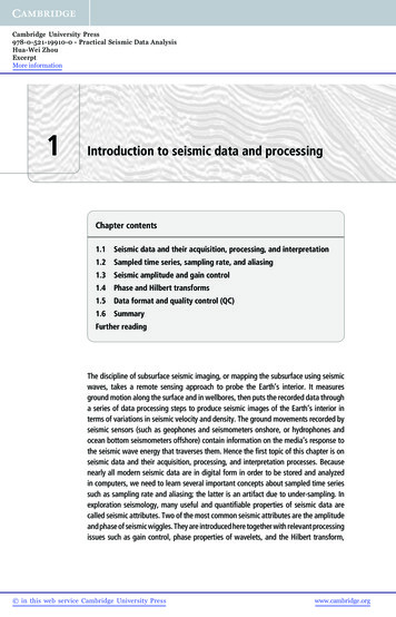
Cambridge University Press978-0-521-19910-0 - Practical Seismic Data AnalysisHua-Wei ZhouExcerptMore information6Practical Seismic Data Analysis100019000500189000-500Crossline offset (m)18800 18700Crossline 0Crosslinedirection17600Inlinedirection1800018400 18800Inline (m)(a)19200 19600050010001500Inline offset (m)2000(b)Figure 1.5 Map views of a three-streamer acquisition from the North Sea (Biondi, 2004).(a) Locations of shots (asterisks) and receivers (dots) for two consecutive shot gathers.(b) Offsets of 1000 traces, randomly selected.the orientations of the shot lines are often perpendicular to the orientations of the receiverlines in order to maximize the azimuthal coverage of each swath, which is a patch of arearecorded by an array of sensors at one time. Typically there is an inline direction alongwhich the spatial sampling is denser than the perpendicular crossline direction. The inlineis often along the receiver line direction, like that shown in Figure 1.4a, because the spacingbetween receivers is typically denser than the spacing between shots. In the case of irregulardistributions of shots and receiver lines, however, the inline direction may be decided basedon the distribution of midpoints of data, like that shown in Figure 1.5b.Sometimes special layouts of shot and receivers are taken to optimize the seismic illumination. Figure 1.6 shows an example of a special 3D seismic survey geometry over theVinton salt dome in southwest Louisiana. The survey placed receivers along radial linesand shots in circular geometry centered right over the subsurface salt diapir. In most appliedsciences, quality and cost are the two main objectives that often conflict with each other,and the cost is in terms of both money and time. Because geophones today are connectedby cables, they are most effectively deployed in linear geometry, such as along the radiallines in this example. The sources here were Vibroseis trucks which can easily be run alongthe circular paths. Similarly, in carrying out seismic data processing projects, we need tosatisfy both the quality and cost objectives.1.1.4SNR and CMP stackingWith respect to the objectives of each project, geophysical data may contain relevantinformation – the signal – and irrelevant components – noise. A common goal for digitaldata processing in general and for seismic data processing in particular is to improve thesignal-to-noise ratio or SNR. In seismology the SNR is often expressed as the ratio betweenthe amplitude of the signal portion and the amplitude of the noise portion of seismic traces. in this web service Cambridge University Presswww.cambridge.org
Cambridge University Press978-0-521-19910-0 - Practical Seismic Data AnalysisHua-Wei ZhouExcerptMore information7Introduction to seismic data and processingPowerlineRoadNFigure 1.6 Map view of a 3D seismic survey over the Vinton salt dome in west Louisiana. Thestraight radial lines denote receiver positions, and the circular lines denote shot positions. Thegeometry of the shot and receiver layout is designed to optimize the coverage of reflectionwaves from the boundary of the underlying salt dome.Box 1.1 Why use CMP stacking and what are the assumptions?The main reason is to improve the SNR and focus the processing on the most coherentevents in the CMP gather. CMP stacking is also a necessary step for post-stack migrationwhere each stacked trace is regarded as a zero-offset trace. The assumption is there is alayer-cake depth velocity model, at least locally within each CMP gather.In practice the meaning of signal versus noise is relative to the objectives of the study andthe chosen data processing strategy. Similarly, the meanings of raw data versus processeddata may refer to the input and output of each specific processing project. The existenceof noise often demands that we treat seismic data from a statistical point of view.Common midpoint (CMP) stacking (see Box 1.1) refers to summing up those seismictraces whose reflections are expected to occur at the same time span or comparable reflectiondepths. The main motivation for such stacking is to improve the SNR. In fact, stacking isthe most effective way to improve the SNR in many observational sciences. A midpointfor a source and receiver pair is simply the middle position between the source and receiver.In a layer-cake model of the subsurface, the reflection points on all reflectors for a pair ofsource and receiver will be located vertically beneath the midpoint (Figure 1.7). Since thelayer-cake model is viewed as statistically the most representative situation, it is commonlytaken as the default model, and the lateral positions of real reflectors usually occur quiteclose to the midpoint. Consequently on cross-sections we usually plot seismic traces attheir midpoints. Clearly, many traces share the same midpoint. In the configuration of CMPbinning, the number of traces in each CMP bin is the fold.It is a common practice in seismic data processing to conduct CMP stacking to producestacked sections. Thus, reflection seismic data can be divided into pre-stack data and in this web service Cambridge University Presswww.cambridge.org
Cambridge University Press978-0-521-19910-0 - Practical Seismic Data AnalysisHua-Wei ZhouExcerptMore information8Practical Seismic Data AnalysishSMhRhSMv1v2Rv2v3v3vn(a)hv1vn(b)Figure 1.7 Reflection rays (black lines) from a source S to a receiver R in (a) a layer-cakemodel; and (b) a model of dipping layers. All reflection points are located vertically beneaththe midpoint M in the layer-cake model.post-stack data, and processing can be divided into pre-stack processing and post-stackprocessing. The traditional time sections are obtained through the process of stackingand then post-stack migration. Modern processing often involves pre-stack processingand migration to derive depth sections that have accounted for lateral velocity variationsand therefore supposedly have less error in reflector geometry and amplitude. One canalso conduct depth conversion from time section to depth section using a velocity–depthfunction. Post-stack seismic processing is cheaper and more stable but less accurate thanpre-stack seismic processing. In contrast, pre-stack seismic processing is more costly, oftenunstable, but potentially more accurate than post-stack seismic processing.1.1.5Data processing sequenceThe primary objective of this book is to allow the reader to gain a comprehensive understanding of the principles and procedures of common seismic data processing and analysis techniques. The sequence of processing from raw seismic data all the way to finalforms ready for interpretation has evolved over the years, and many general aspects ofthe sequence have become more-or-less conventional. It is a non-trivial matter to designa proper sequence of seismic data processing, called a processing flow. Figure 1.8 showsan example of a processing flow for reflection seismic data more than 30 years ago (W. A.Schneider, unpublished class notes, 1977). The general procedure shown in this figure stillholds true for today’s processing flow for making post-stack sections.The goal of seismic data processing is to help interpretation, the process of decipheringthe useful information contained in the data. The task is to transfer the raw data into a formthat is optimal for extracting the signal. The word “optimal” implies making the best choiceafter considering all factors. Hence we need to make decisions in the process of seismicdata analysis. All methods of seismic data analysis rely on physical and geological theoriesthat tie the seismic data and the geological problem together. For instance, a problem ofinferring aligned fractures may involve the theory of seismic anisotropy. The subsequentdata processing will attempt to utilize this theory to extract the signal of the fracture in this web service Cambridge University Presswww.cambridge.org
Cambridge University Press978-0-521-19910-0 - Practical Seismic Data AnalysisHua-Wei ZhouExcerptMore information9Introduction to seismic data and processinga. Data ConditioningInput: Field tapes1. Gain removal G-1(t)2. Source array stack3. Source correction (Vibroseis, etc.)4. True amplitude recovery5. Trace editing6. Wavelet deconvolution7. Reverberation deconvolution8. CDP sortingOutput: CDP fileb. Parameter AnalysisInput: CDP file1. Statics correction2. Stacking velocity analysis3. Residual statics analysis / Velocityinterpretation4. QC stackOutput: CDP, statics, & velocity filesc. Data EnhancementInput: CDP, statics, & velocity files1. NMO & statics corrections2. CDP stack3. Earth absorption compensation4. Time variant band-pass filtering5. Display of time sectionOutput: Time sectiond. Migration / Depth ConversionInput: CDP & velocity files1. Time migration2. Migration velocity analysis3. Time migration & depth conversion4. Depth migrationOutput: Migrated volumese. Modeling & InterpretationProduce reservoir models based onseismic, geology, & well dataf. Exploration Decision Making1. Where, when, & how to drill?2. Analysis risks & economicsFigure 1.8 A general processing flow, after Schneider (unpublished class notes from 1977).Steps c, d, and e are usually iterated to test different hypotheses. Pre-stack processing is oftenconducted after a post-stack processing to help the velocity model building process. There arealso reports of pre-stack processing using limited offsets to increase the efficiency.orientation according to the angular variation of traveling speed, and to suppress the noisethat may hamper the signal extraction process.Exercise 1.11. How would you estimate the fold, the number of the source-to-receiver midpoints ineach CMP bin, from a survey map like that shown in Figure 1.6? Describe yourprocedure and assumptions.2. As shown in Figure 1.7, the shapes of reflection raypaths tend to resemble the letter“U” rather than the letter “V”. Explain the reason behind this phenomenon.3. Update the processing flow shown in Figure 1.8 by finding and reading at least twopapers published within the past 10 years. What happened to those processing steps inFigure 1.8 that are missing from your updated processing flow? in this web service Cambridge University Presswww.cambridge.org
Cambridge University Press978-0-521-19910-0 - Practical Seismic Data AnalysisHua-Wei ZhouExcerptMore information10Practical Seismic Data Analysis02Time [s]4680.736Distance [km]91215Figure 1.9 A common shot gather from an offshore seismic survey.1.2Sampled time series, sampling rate, and aliasing.Through their propagation history, seismic waves vary in a continuous manner in both temporal and spatial dimensions. However, measurements of seismic data need to be sampledinto digital form in order to be stored and processed using computers. At the acquisitionstage each trace of seismic wiggles has been digitized at a constant sample interval, suchas 2 ms (milliseconds). The resulted string of numbers is known as a time series, wherethe number represents the amplitude of the trace at the corresponding sample points. In thefollowing, some basic properties of the sampled time series are introduced.1.2.1Sampled time seriesFigure 1.9 shows an example of offshore seismic data for which the streamer of hydrophonesis nearly 20 km long. We treat each recorded seismic trace as a time series, which isconceptualized as an ordered string of values, and each value represents the magnitudeof a certain property of a physical process. The word “time” here implies sequencing orconnecting points in an orderly fashion. A continuous geological process may be sampledinto a discrete sequence called a sampled time series. Although the length of the sampleis usually finite, it may be extrapolated to infinity when necessary. All the data processingtechniques discussed in this book deal with sampled time series. A 1D time series is usuallytaken to simplify the discussion. However, we should not restrict the use of time series tojust the 1D case, because there are many higher-dimensional applications. in this web service Cambridge University Presswww.cambridge.org
1 Introduction to seismic data and processing Chapter contents 1.1 Seismic data and their acquisition, processing, and interpretation 1.2 Sampled time series, sampling rate, and aliasing 1.3 Seismic amplitude and gain control 1.4 Phase and Hilbert transforms 1.5 Data fo