Transcription
https://doi.org/10.5194/acp-2022-416Preprint. Discussion started: 14 July 2022c Author(s) 2022. CC BY 4.0 License.Airborne glyoxal measurements in the marine and continentalatmosphere: Comparison with TROPOMI observations and EMACsimulationsFlora Kluge1 , Tilman Hüneke1,a , Christophe Lerot2 , Simon Rosanka3 , Meike K. Rotermund1 , DomenicoTaraborrelli3 , Benjamin Weyland1 , and Klaus Pfeilsticker1,41Institute of Environmental Physics, Heidelberg University, Heidelberg, GermanyAtmospheric reactive gases, Royal Belgian Institute for Space Aeronomy (BIRA-IASB), Brussels, Belgium3Forschungszentrum Jülich, Institute for Energy and Climate Research: Troposphere (IEK-8), Jülich, Germany4Heidelberg Center for the Environment, Heidelberg University, Heidelberg, Germanyanow with Encavis AG, Hamburg, Germany2Correspondence: Flora Kluge(fkluge@iup.uni-heidelberg.de)Abstract. We report on airborne Limb and Nadir measurements of vertical profiles and total vertical column densities (VCDs)of glyoxal (C2 H2 O2 ) in the troposphere, which were performed from aboard the German research aircraft HALO (High Altitude and LOng Range) in different regions and seasons around the globe between 2014 and 2019. The airborne Nadir andintegrated Limb profiles excellently agree among each other. Our airborne observations are further compared to collocated gly5oxal measurements of the TROPOspheric Monitoring Instrument (TROPOMI), with good agreement between both data setsfor glyoxal observations in (1) pristine terrestrial, (2) pristine marine, (3) mixed polluted, and (4) biomass burning affected airmasses with high glyoxal concentrations. Exceptions from the overall good agreement are observations of (1) faint and agedbiomass burning plumes over the oceans and (2) of low lying biomass burning or anthropogenic plumes in the terrestrial ormarine boundary layer, both of which contain elevated glyoxal that is mostly not captured by TROPOMI. These differences10of airborne and satellite detected glyoxal are most likely caused by the overall small contribution of plumes of limited extentto the total atmospheric absorption by glyoxal and the difficulty to remotely detect weak absorbers located close to low reflective surfaces (e.g. the ocean in the visible wavelength range), or within dense aerosol layers. Observations of glyoxal inaged biomass burning plumes (e.g. observed over the Tropical Atlantic off the coast of West Africa in summer 2018, off thecoast of Brazil by the end of the dry season 2019, and the East China Sea in spring 2018) could be traced back to related15wildfires, such as a plume crossing over the Drake Passage that originated from the Australian bushfires in late 2019. Ourobservations of glyoxal in these over days aged biomass burning plumes thus confirm recent findings of enhanced glyoxal andpresumably secondary aerosol (SOA) formation in aged wildfire plumes from yet to be identified longer-lived organic precursor molecules (e.g. aromatics, acetylene, or aliphatic compounds) co-emitted in the fires. Further, elevated glyoxal (median44 ppt) as compared to other marine regions (median 10–19 ppt) is observed in the boundary layer over the tropical oceans,20well in agreement with previous reports. The airborne data sets are further compared to glyoxal simulations performed withthe global atmosphere-chemistry model EMAC (ECHAM/MESSy Atmospheric Chemistry). When using an EMAC setup that1
https://doi.org/10.5194/acp-2022-416Preprint. Discussion started: 14 July 2022c Author(s) 2022. CC BY 4.0 License.resembles recent EMAC studies focusing on complex chemistry, reasonable agreement is found for pristine air masses (e.g. theunperturbed free and upper troposphere), but notable differences exist for regions with high emissions of glyoxal and glyoxalproducing volatile organic compounds (VOC) from the biosphere (e.g. the Amazon), mixed emissions from anthropogenic25activities (e.g. over continental Europe, the Mediterranean and East China Sea), and potentially from the sea (e.g. the tropicaloceans). Also, the model tends to largely under-predict glyoxal in city plumes and aged biomass burning plumes. The potentialcauses for these differences are likely to be multifaceted, but they all point to missing glyoxal sources from the degradation ofthe cocktail of (potentially longer-chained) organic compounds emitted from anthropogenic activities, biomass burning, andfrom the organic micro-layer of the sea.301IntroductionGlyoxal (C2 H2 O2 ), the simplest α-dicarbonyl, has significant importance in air quality and climate, due to its role as anintermediate in the oxidation of hydrocarbons (e.g. Finlayson-Pitts and J. N. Pitts (1986); Volkamer et al. (2001); Fu et al.(2008); Myriokefalitakis et al. (2008); Vrekoussis et al. (2009); Nishino et al. (2010); Li et al. (2016); Chan Miller et al.(2017); Wennberg et al. (2018)) and as an important precursor for secondary organic aerosol (SOA) formation and thus for35the aerosol forcing of climate (e.g. Jang and Kamens (2001); Liggio et al. (2005b); Volkamer et al. (2007); Lim et al. (2013);Knote et al. (2014); Kim et al. (2022)).The global sources of glyoxal are estimated to 45 Tg a 1 (Fu et al., 2008), and the largest single source ( 47%) is believedto be the oxidation of isoprene emitted by vegetation (e.g. Myriokefalitakis et al. (2008); Li et al. (2016); Chan Miller et al.(2017); Wennberg et al. (2018)). Precursor molecules of glyoxal, that are mostly (but not exclusively) anthropogenically emitted40include alkenes, acetylene, various aromatics, monoterpenes and other volatile organic compounds (VOCs) with differentyields (Volkamer et al., 2001; Fu et al., 2008; Nishino et al., 2010; Taraborrelli et al., 2021). A recent study found that below2 km altitude, the production of glyoxal in the city plume of the Seoul Metropolitan Area (South Korea) was mainly causedby the oxidation of aromatics ( 59%) initiated by hydroxyl radicals (Kim et al., 2022). Glyoxal is also directly emitted inconsiderable amounts by biomass burning, together with a suite of organic glyoxal precursor molecules in largely seasonal and45regional varying amounts (e.g. Andreae (2019); Akagi et al. (2011); Stockwell et al. (2015); Zarzana et al. (2017, 2018); Klugeet al. (2020)).The predominant photochemical loss process of glyoxal is photolysis, and to a lesser degree reactions with OH radicals(Koch and Moortgat, 1998; Volkamer et al., 2005a; Tadić et al., 2006; Fu et al., 2008; Wennberg et al., 2018). Uptake ofglyoxal on aerosols in polluted environments as well as on cloud particles can eventually compete with its photochemical50losses (e.g. Volkamer et al. (2007); Kim et al. (2022)), primarily due to its high water solubility (e.g. Zhou and Mopper (1990);Kroll et al. (2005); Ip et al. (2009); Kampf et al. (2013)), and oligomerization potential (e.g. Whipple (1970); Liggio et al.(2005a); Loeffler et al. (2006); Galloway et al. (2009)). While the global mean lifetime of glyoxal is less than a few hours, inthe sunlit polluted atmosphere it can be as short as half an hour due to photolysis, reactions with OH and heterogeneous uptake(Volkamer et al., 2007; Kim et al., 2022).2
https://doi.org/10.5194/acp-2022-416Preprint. Discussion started: 14 July 2022c Author(s) 2022. CC BY 4.0 License.55Accordingly, due to the varying source strength of glyoxal and its short lifetime, in pristine air its mixing ratios may rangefrom several ppt to a few 10 ppt. For example, 7–23 ppt of glyoxal were found over the South Pacific (Lawson et al., 2015), orup to 10 ppt at the Cape Verde Atmospheric Observatory (CVAO, Sao Vicente island) over the Tropical Atlantic (Walker et al.,2022). Further, Mahajan et al. (2014) reported an average glyoxal mixing ratio of 25 ppt from 10 field campaigns over the openoceans in different parts of the world. Contrary to the low glyoxal mixing ratios observed in the pristine marine environment,60in polluted air glyoxal mixing ratios may reach several 100 ppt (e.g. Lee et al. (1998); Volkamer et al. (2005a, 2007); Fu et al.(2008); Sinreich et al. (2010); Baidar et al. (2013); Kaiser et al. (2015); Volkamer et al. (2015); Chan Miller et al. (2017); Klugeet al. (2020); Kim et al. (2022), and others), or even up to 1.6 ppb, as found over a tropical rainforest with large emissions ofisoprene in South-East Asia (MacDonald et al., 2012).Glyoxal is detectable from space by satellites applying a similar technique (DOAS, Differential Optical Absorption Spec-65troscopy, (Platt and Stutz, 2008)) as used for the airborne data in this study. Accordingly, since the first glyoxal observationsof UV/vis Nadir observing spectrometers (e.g. from the Scanning Imaging Absorption Spectrometer for Atmospheric Chartography (SCIAMACHY); Wittrock et al. (2006)), numerous studies with ever increasing observation capabilities and spatialresolution have been reported for space-borne measurements of vertical column densities (VCD) of glyoxal (e.g. from theinstruments OMI (Ozone Monitoring Instrument), and TROPOMI (TROPOspheric Monitoring Instrument; Stavrakou et al.70(2009a); Vrekoussis et al. (2009); Lerot et al. (2010); Vrekoussis et al. (2010); Chan Miller et al. (2014); Alvarado et al.(2020, 2014); Lerot et al. (2021)), and many others). These space-borne measurements provided a wealth of new informationon the worldwide sources, occurrence and abundance of glyoxal and its relation to the photochemistry of VOCs and aerosols(e.g. Fu et al. (2008)).Simultaneous measurements of formaldehyde (CH2 O) and glyoxal by satellites and airborne instruments complemented by75modelling have been exploited to study its different sources (e.g. Stavrakou et al. (2009b); Lerot et al. (2010); Boeke et al.(2011); Chan Miller et al. (2014); Bauwens et al. (2016); Stavrakou et al. (2016)), to elucidate the secondary aerosol formation from carbonyls (typically in the background atmosphere) as well as its fate in biomass burning plumes (Knote et al.,2014; Li et al., 2016; Lim et al., 2019), and even more recently, to estimate the organic aerosol abundance (Liao et al., 2019).Ground-based, air-, and space-borne simultaneous measurements of formaldehyde and glyoxal and of the [C2 H2 O2 ]/[CH2 O]80ratio were further helpful to study the glyoxal yield from isoprene oxidation in relation to formaldehyde, to specify the varioushydrocarbon glyoxal precursors, to investigate the anthropogenic impact on rural photochemistry, and more recently to investigate the sources of glyoxal and the chemical evolution of VOCs in biomass burning plumes (e.g. Lee et al. (1998); Wittrocket al. (2006); Vrekoussis et al. (2010); DiGangi et al. (2012); MacDonald et al. (2012); Kaiser et al. (2015); Bauwens et al.(2016); Li et al. (2016); Chan Miller et al. (2017); Zarzana et al. (2017); Hoque et al. (2018); Behrens et al. (2019); Alvarado85et al. (2020); Kluge et al. (2020)).Together with respective photochemical model simulations, some of the glyoxal observations point to deficits in our presentunderstanding of atmospheric glyoxal. This includes (1) the observation of unexpected large glyoxal concentrations in the marine boundary layer of the Eastern Pacific up to 3000 km from the continental coast by ship-borne (up to 140 ppt; Sinreich et al.(2010)) and airborne measurements (32 – 36 ppt; Volkamer et al. (2015)). These measurements revealed a yet unknown ma3
https://doi.org/10.5194/acp-2022-416Preprint. Discussion started: 14 July 2022c Author(s) 2022. CC BY 4.0 License.90rine source of glyoxal, possibly from ozone-driven reactions with the organic microlayer at the sea surface, which in idealisedseawater laboratory experiments have been shown to produce glyoxal (Zhou et al., 2014), and/or secondary formation fromoxidised VOC (OVOC) precursor molecules, such as acetaldehyde, acetylene, and others (Wang et al., 2019). (2) Unlike forformaldehyde, the models had still varying success in reproducing the glyoxal VCDs (Myriokefalitakis et al., 2008; Stavrakouet al., 2009a; Lerot et al., 2010). Moreover, in comparisons of satellite measurements from SCIAMACHY and GOME-2,95several studies have found that the models underestimate global glyoxal emissions, when not considering additional biogenicsources (Myriokefalitakis et al., 2008; Stavrakou et al., 2009a; Lerot et al., 2010). (3) Finally, a recent study by Alvarado et al.(2020) found unexpected large amounts of glyoxal (and formaldehyde) in several days old air masses originating from Canadian wildfires in August 2018, which can only be reconciled with the source strength and lifetime of glyoxal if consideringsecondary formation of glyoxal from OVOCs that were co-emitted from the fires.100Here, we report on airborne measurements of glyoxal concentrations (Limb) and total vertical column densities (Nadir)performed during eight missions from the German research aircraft HALO (High Altitude and Long Range) in different regionsof the globe between 2014 and 2019. The measurements are able to provide novel information on the sources and fate of glyoxalin the atmosphere and address aspects on some open issues in glyoxal and VOC research as outlined above. This includes novelinsights into the amount and vertical distribution of glyoxal in the polluted terrestrial (South America, Europe, East Asia),105polluted marine (East China and Mediterranean Sea, South American and West African coastlines), pristine terrestrial (SouthAmerica), and pristine marine (South and North Atlantic) atmosphere. The observations may thus not only serve to validaterespective satellite observations, but also simulations of atmosphere-chemistry models to better assess the global budget ofglyoxal, the role of glyoxal for the atmospheric oxidation capacity and its contribution to secondary aerosol formation. Finally,our glyoxal profiles and VCDs measured in different regions and seasons may also serve as input for air mass calculations110necessary to better infer total atmospheric column densities of glyoxal from the various satellite observations (e.g. GOME-2,SCIAMACHY, OMI, and TROPOMI).In the present study, the airborne Nadir glyoxal measurements are corroborated and validated against near collocated observations of the TROPOMI satellite instrument. The Limb and Nadir measurements are further compared to simulations of theglobal ECHAM/MESSy Atmospheric Chemistry (EMAC) model, of which further details are presented in a companion paper115(S. Rosanka et al., in preparation). The specific scientific questions addressed in both publications include: (1) the marine andterrestrial background of glyoxal and its potential sources, (2) the sources of glyoxal in the polluted atmosphere, (3) secondarily formed glyoxal in biomass burning plumes, (4) the global budget of glyoxal, and (5) its potential contribution to secondaryaerosol formation.The paper is organized as follows. Section 2 briefly describes the measurement technique and involved methods used in the120present study. Section 3 reports on the deployment and measurements of the mini-DOAS instrument on eight missions of theHALO research aircraft into different regions from 2014 until 2019. Chapter 4 presents the airborne concentration and VCDmeasurements of glyoxal. The latter are then compared to collocated total atmospheric column density observations of glyoxalmade from the TROPOMI instrument. Finally, both airborne data sets -glyoxal concentrations and VCDs- are compared to4
https://doi.org/10.5194/acp-2022-416Preprint. Discussion started: 14 July 2022c Author(s) 2022. CC BY 4.0 License.simulations of the global atmosphere-chemistry model EMAC. Chapter 5 discusses the major findings and results, and chapter1256 concludes and summarises the study.2Instruments and methods2.1The airborne mini-DOAS measurementsThe airborne mini-DOAS measurements of UV/vis/near-IR absorbing gases involve: (1) simultaneous measurements of Limband Nadir scattered skylight, (2) the Differential Optical Absorption Spectroscopy (DOAS) analysis of the measured skylight130spectra for the target gases (Platt and Stutz, 2008), and (3) forward radiative transfer modelling of the observations using theMonte Carlo model McArtim (Deutschmann et al., 2011). In a last step, trace gas concentrations are inferred from the Limbobservations by scaling the measured slant column densities (SCDs) using simultaneously measured SCDs of a scaling gas ofknown concentration (e.g. O3 ), or calculated (clear sky) extinction of the collisional complex O2 O2 , or briefly (O4 ; Hüneke(2016); Hüneke et al. (2017); Stutz et al. (2017); Werner et al. (2017); Kluge et al. (2020); Rotermund et al. (2021)). For the135Nadir observations, air mass factors are simulated using the same radiative transfer model (McArtim) to infer VCDs from themeasured SCDs.The presented study focuses on the Nadir and Limb measurements of O4 and C2 H2 O2 by the mini-DOAS instrument madefrom aboard the German research aircraft HALO during a total of 72 research flights on eight scientific missions coveringdifferent regions of the globe. The processing of the measured data is mainly based on our previous study on O4 , CH2 O, and140C2 H2 O2 (Kluge et al., 2020). Since some aspects of the data processing changed since then, necessary details on these changesand refinements are provided in the following.2.1.1The mini-DOAS instrumentThe mini-DOAS instrument is a UV/vis/near-IR six channel optical spectrometer, which has been operated on board theHALO research aircraft since 2011. It detects and spectrally analyses Nadir and Limb scattered sunlight in the UV (310–145440 nm, FWHM 0.47 nm), visible (420–640 nm, FWHM 1.1 nm) and near-infrared (1100–1680 nm, FWHM 10 nm)wavelength ranges (Hüneke, 2016; Hüneke et al., 2017). The six telescopes (FOV 0.5 3.15 ) collect the skylight fromfixed Nadir and Limb viewing geometries each in the UV, visible and near-IR channel. The limb telescopes can be adjustedto varying elevation angles ( 5 to -90 ) when commanded, but are normally aligned with a rate of 10 Hz at -0.5 below thehorizon to compensate for the changing roll angle of the aircraft. Glass fibre bundles transmit the collected skylight to six optical150spectrometers, assembled in an evacuated (10 5 mbar) and thermostated housing (at 1 C) in the otherwise umpressurizedand uninsulated boiler room of the aircraft. In the Limb geometry, the mini-DOAS instrument probes air-masses perpendicularto the aircraft’s flight direction on the starboard side, with typical photon path lengths in the visible wavelength range rangingfrom 10 km (at 2 km altitude) to about 100 km at the maximum flight altitude of the aircraft around 15 km, depending onthe wavelength, aerosol concentration and cloud cover (see Fig. 2 in Kluge et al. (2020) and below). In the Nadir observation5
https://doi.org/10.5194/acp-2022-416Preprint. Discussion started: 14 July 2022c Author(s) 2022. CC BY 4.0 License.Table 1. Trace gas absorption cross sections used for the spectral retrieval. For H2 O, gas phase (g) as well as liquid phase (l) absorptioncross sections are used.No.AbsorberTemperature [K]ReferenceUncertainty [%]1aO4273Thalman and Volkamer (2013)41bO4293Thalman and Volkamer (2013)42aO3203Serdyuchenko et al. (2014)32bO3223Serdyuchenko et al. (2014)32cO3273Serdyuchenko et al. (2014)33NO2294Vandaele et al. (1998)34aH2 O (g)293Rothman et al. (2009)84bH2 O (g)296Polyansky et al. (2018)14cH2 O (l)295Pope and Fry (1997)15CH2 O293Chance and Orphal (2011)106C2 H2 O2296Volkamer et al. (2005b)3Table 2. Details of the DOAS spectral analysis for the various trace gases.SpectrometerTarget gasSpectral interval [nm]LimbO4460–4901a, 2a, 2c, 3, 4a21, 2, 3, 4, 5, 6, 7, 8LimbC2 H2 O2420–439 and 447–4651a, 2c, 3, 4a, 621C2 H2 O2435–4601b, 2b, 3, 4b, 4c, 634, 6, 8C2 H2 O2430–4601b, 2b, 3, 4b, 4c, 632, 3, 5, 7C2 H2 O2435–4601b, 2b, 3, 4b, 4c, 633, 4, 5, 6, 7, 8NadirFitted absorbers (see Table 1)Polyn.Additional parameters for all spectral retrievals are (1) Offset spectrum; (2) Ring spectrum; (3) Ring spectrum multiplied by λMission (i)4(i): ACRDICON-CHUVA (1), OMO (2), EMeRGe-EU (3), WISE (4), EMeRGe-Asia (5), CoMet (6), CAFE-Africa (7), SouthTRAC (8).155mode, the instrument measures the atmospheric column density of the targeted gases below the aircraft with a rectangularfoot print of 600 m cross-track and several km along-track (FOV 3.15 0.38 ), depending on the flight altitude, cruisingvelocity (typically 200 m s 1 in the upper troposphere) and signal integration time (up to 1 min). Further, an IDS uEyecamera (FOV 46 ) aligned with the Limb telescopes provides images of the sampled atmosphere at 1 Hz resolution.More details of the instrument design, its major features, deployment on the HALO aircraft, the measurement method, the160spectral retrieval and data processing can be found in Hüneke et al. (2017).2.1.2The spectral retrievalThe measured skylight spectra are analysed using the DOAS technique (Platt and Stutz, 2008). The retrieval details such aswavelength ranges, included trace gases and fitting parameters for each gas are provided in Tables 1 and 2.6
https://doi.org/10.5194/acp-2022-416Preprint. Discussion started: 14 July 2022c Author(s) 2022. CC BY 4.0 License.The spectral retrieval settings of the Limb and Nadir glyoxal observations are based on the recent TROPOMI glyoxal165analysis from Lerot et al. (2021), in support of a better comparability of both data sets (see Sect. 4.2). Unlike the TROPOMIglyoxal retrieval, the mini-DOAS measurements were not found to be significantly affected by changing NO2 concentrations,therefore only a single NO2 absorption cross section (at a warmer temperature) is included in our analysis to account for thetropospheric NO2 absorption. A noteworthy difference to our recent glyoxal retrieval of the ACRIDICON-CHUVA data is theuse of a continuous fitting window ranging from 430 nm (or 435 nm for campaigns 4, 6, 8, and all Nadir observations) to170460 nm, instead of employing two simultaneous retrieval windows from 420 nm to 439 nm and 447 nm to 465 nm (Klugeet al., 2020). The comparison of the spectral retrieval employing both wavelength ranges (i.e. when performing the spectralanalysis for each spectrum with both wavelength ranges) yields an improvement in the spectral residuum and signal to noiseratio when using the continuous retrieval window, however with comparable dSCDs from both approaches. For the processingof the data from different missions, minor adjustments to the retrieval settings (e.g. lower end of the analysed wavelength range175or temperatures of the included absorption cross sections) are applied when needed. Primarily, these adjustments are necessaryto compensate for mechanical modifications of the instrument and hence of the optical imaging (e.g. due to a fibre bundlereplacement, which causes changes in the lower wavelength limit of the spectrometers) as well as due to the largely changingambient conditions during the different research missions.In particular for Nadir observations in a moist atmosphere and above the ocean, the DOAS analysis of glyoxal is challenging180due to its low optical density ( 10 4 ) and proximity of the main absorption bands to the much stronger 7ν absorption band ofwater vapour (optical density on the order of 10 1 (Wei et al., 2019)). Therefore, for such observations, 5–150 consecutivelymeasured skylight spectra are co-added in order to minimise potential spectral interferences while optimising the signal tonoise, at the expense of enlarging the footprint of the affected measurements (as discussed in detail below).Since the DOAS method infers a differential slant column density dSCD relative to a solar Fraunhofer reference spectrum185SCDref , the total slant column SCD has to be inferred fromSCD SCDref dSCD.(1)For the glyoxal retrieval, SCDref is determined from a Limb measurement at high altitudes above which insignificant (or no)glyoxal is expected, or if a sufficient flight altitude was not reached (EMeRGe-Europe and EmeRGe-Asia missions) by usinga reference from a different research flight which fulfills the above condition. For the retrieval of the O4 extinction, SCDref is190determined using a high resolution solar reference spectrum (Thuillier et al., 1998).The mini-DOAS detection limit for glyoxal dSCDdl is 2.6 · 1014 molec cm 2 (Platt and Stutz, 2008). Depending on SCDrefand the related air mass factors (Sect. 2.1.3) and hence flight altitude, for Limb measurements, this results in a detectionlimit ranging from 1 ppt (during clear skies, for a light path of about 100 km at maximum cruising altitude of the aircraft)up to several 100 ppt (for very short line-of-sight photon paths, e.g. in dense clouds; Kluge et al. (2020)). For the Nadir195measurements, the typical detection limit [VCDdl ] is 1.5 · 1014 molec cm 2 , but depending on the flight altitude and cloudcover and thus columnar air mass factor, it can be as low as 6.7 · 1013 molec cm 2 or as large as 2.6 · 1014 molec cm 2 .7
https://doi.org/10.5194/acp-2022-416Preprint. Discussion started: 14 July 2022c Author(s) 2022. CC BY 4.0 License.2.1.3Retrieval of concentrations (Limb) and vertical column densities (Nadir)The following section discusses the conversion of the inferred SCDs to mixing ratios (Limb measurements) and to total verticalcolumn densities (Nadir measurements).200The Limb measured slant column densities SCDlimb are converted into trace gas mixing ratios using the O4 -scaling method,as described in detail in Hüneke (2016); Hüneke et al. (2017); Stutz et al. (2017); Werner et al. (2017); Kluge et al. (2020).Accordingly, the concentration of a trace gas [X] at flight altitude j is inferred from SCDlimb,X by comparing the measuredoptical depth SCDlimb,O4 with the calculated clear sky extinction [O4 ]j and taking into account radiative transfer-based correction factors αXj and αO4,j ) to quantify the optical characteristics (e.g. aerosol and cloud cover) of the radiative transfer during205each single measurement:[X]j αXj SCDlimb,X·· [O4 ]j .αO4,j SCDlimb,O4(2)This approach is justified based on the equivalence theorem in optics (Irvine, 1963), which states that for a given wavelength,the photon path length distribution and hence the mean photon path lengths are the same for weak absorbers with similaratmospheric distributions. Evidently, this criterion is reasonably well approximated when using O4 as scaling gas for all trace210gases with sources at the ground and sinks in the troposphere, such as C2 H2 O2 . The remaining differences in the profileshapes of the target (X) and scaling gas (O4 ) and their centre wavelengths of absorption are accounted for by the so called αfactors. The α-factors express the fraction of absorption within the line-of-sight at the measurement altitude relative to the totalatmospheric absorption, which may differ slightly for the gas of interest compared to the scaling gas due to their different profileshapes and absorption wavelengths. The α-factors are simulated using the McArtim radiative transfer model (Deutschmann215et al., 2011). For the simulation, in a first step a priori profiles of glyoxal are used based on previous mini-DOAS measurementsin similar atmospheric conditions (clean and polluted terrestrial air, remote marine air et cetera), and subsequently iterated untilconvergence is achieved (see below). In the following, the robustness of the iterative approach is described and tested. In a firststep, the RT model is run using an a priori glyoxal profile obtained during previous missions and assuming an exponentiallydecaying profile above the maximum flight altitude. Secondly, a modelled a priori glyoxal profile is used based on simulations220from the global chemical transport model MAGRITTE (Model of Atmospheric composition at Global and Regional scalesusing Inversion Techniques for Trace gas Emissions). This model is used e.g. to calculate air mass factors for the TROPOMIretrieval (e.g. Bauwens et al. (2016); Lerot et al. (2021)). Here, the simulated MAGRITTE glyoxal a prioris are averaged alonga research flight track over central Europe on 15 May 2018. Both a prioris -simulated and measured- show notable differencesin their absolute mixing ratios as well as in their profile shape (Fig. 1, panels a and b). In the following, iterations of the225radiative transfer simulation are performed for the flight on 15 May 2018 using consecutively resulting profiles from bothapproaches as new a priori profiles (Fig. 1, panels a and b). Evidently, even strongly diverging a priori profiles converge wellafter the first iteration to a common profile constrained by the measured SCDs within the error margins. After four iterations,no notable changes are discernible in the obtained a priori profiles as well as in the resulting mixing ratios (Fig. 1, panel c), thusdemonstrating the robustness of the iteration with respect to the a priori profile assumptions. This insensitivity of the resulting230profiles towards the assumed a priori profile is a direct consequence of the applied scaling method, because all a priori profiles8
https://doi.org/10.5194/acp-2022-416Preprint. Discussion started: 14 July 2022c Author(s) 2022. CC BY 4.0 License.12(a)A priori profilesm10TAltitude [km]T8T0011122VMRm -T3830123244222200VMR84100VMRm -T600VMR10m -T6TDifferenceof results2m612 (c)m -T101mDifference of a prioris00m12 (b)333000-10001002003000-200-1000100200Glyoxal [ppt]Figure 1. Iterations of different a priori glyoxal profiles in α-factor calculations, shown here for the HALO flight on 15 May 2018 (CoMetmission). Starting a priori profiles are a mean glyoxal profile inferred from previous mini-DOAS measurements in polluted continental air(m0 ), and an averaged glyoxal profile simulated by the MAGRITTE model (T0 ) for a TROPOMI overpass over Europe at 13:30 UTC on 15May 2018 (Lerot et al., 2021). These a prioris are used for the first iteration in the α-fact
Airborne glyoxal measurements in the marine and continental . and glyoxal by satellites and airborne instruments complemented by 75 modelling have been exploited to study its different sources (e.g. Stavrakou et al. (2009b); Lerot et al. (2010); Boeke et al. . seawater laboratory experiments have been shown to produce glyoxal (Zhou et al .