WIXLIB

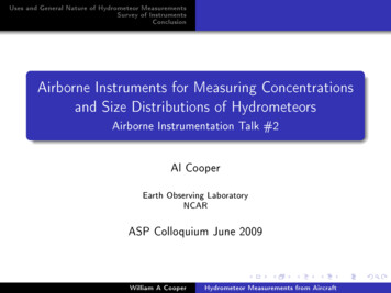
F. Ewald et al.: Calibration of a 35 GHz airborne cloud radar1817of this work is the determination of the receiver sensitivity(Sect. 3.3 and 3.4). In the second part of the paper, the budget calibration is validated by using predicted and measuredocean surface backscatter (Sect. 4.3). In addition, the calibration and system performance for joint flight legs is comparedto the W-band cloud radars like the airborne cloud radarRASTA (Sect. 5.2) and the spaceborne cloud radar CloudSat(Sect. 5.3).Accuracy considerationsIn order to provide scientifically sound interpretations ofcloud radar measurements, a well-calibrated instrument withknown sensitivity is indispensable. Many spaceborne (Delanoë and Hogan, 2008; Deng et al., 2010) or ground-based(Donovan et al., 2000) techniques to retrieve cloud microphysics using millimeter-wave radar measurements requirea well-calibrated instrument. In the case of the CloudSatinstrument, the calibration uncertainty was specified to be 2 dB or better (Stephens et al., 2002). This requirement forabsolute calibration imposed by retrievals of cloud microphysics is further explained in Fig. 1. Under the simplest assumption of small, mono-disperse cloud water droplets, theiso-lines in Fig. 1 represent all combinations of cloud dropleteffective radius and liquid water content with a radar reflectivity of 20 dBz. An increasing retrieval ambiguity, causedby an assumed instrument calibration uncertainty, is illustrated by the shaded areas with 1 dB (green), 3 dB (yellow) and 8 dB (red). To constrain the retrieval space considerably within synergistic radar–lidar retrievals like Cloudnet(Illingworth et al., 2007) or Varcloud (Delanoë and Hogan,2008), the absolute calibration uncertainty has to be significantly smaller than the natural variability of clouds. Sincea reflectivity bias of 8 dB would bias the droplet size by afactor of 2 and the water content by even an order of magnitude, the absolute calibration uncertainty should be at least3 dB or lower. For a systematic 1 dB calibration offset, Protat et al. (2016) still found ice water content biases of 19 %and 16 % in their radar-only retrieval. Since HAMP MIRAdata are used in retrievals of cloud microphysics, the targetaccuracy will be set to 1 dB.An accurate absolute calibration is further motivated byrecent studies (Protat et al., 2009; Hennemuth et al., 2008;Maahn and Kollias, 2012; Ewald et al., 2015; Lonitz et al.,2015; Myagkov et al., 2016; Acquistapace et al., 2017),which used the radar reflectivity provided by almost identical ground-based versions of the same instrument. The installation of the MIRA instrument on many ground-basedcloud profiling sites within ACTRIS (Aerosols, Clouds andTrace gases Research InfraStructure Network; http://www.actris.eu, last access: 10 March 2019) and in the frameworkof Cloudnet is a further incentive for an external calibrationstudy.The need for an external calibration is furthermore encouraged by several studies which already found e 1. Microphysical retrieval uncertainty due to different absolute calibration uncertainties ( 1, 3, 8) for mono-disperse cloudwater droplets according to Mie calculations.of an offset in radar reflectivity when comparing differentcloud radar instruments. In a direct comparison with the WBand (94 GHz) ARM Cloud Radar (WACR), Handwerkerand Miller (2008) found reflectivities around 3 dB smallerfor the Karlsruhe Institute of Technology MIRA, contradicting the reflectivity-reducing effect of a higher gaseous attenuation and stronger Mie scattering at 94 GHz. Protat et al.(2009) could reproduce this discrepancy in a comparisonwith CloudSat, where they found a clear systematic shift ofthe mean vertical profile by 2 dB between Cloudsat and theLindenberg MIRA (CloudSat showing higher values than theLindenberg radar).2The 35 GHz cloud radar on HALOThe cloud radar on HALO is a pulsed Ka-band, polarimetricDoppler millimeter-wavelength radar which is based on prototypes developed and described by Bormotov et al. (2000)and Vavriv et al. (2004). The current system was manufactured and provided by Metek (Meteorologische Messtechnik GmbH, Elmshorn, Germany). The system design andits data processing, including an updated moment estimationand a target classification by Bauer-Pfundstein and Görsdorf(2007), was described in detail by Görsdorf et al. (2015). Themillimeter radar is part of the HALO Microwave Package(HAMP) which will be subsequently abbreviated as HAMPMIRA. Its standard installation in the belly pod section ofHALO with its fixed nadir-pointing 1 m diameter Cassegrainantenna is described in detail by Mech et al. (2014). Its transmitter is a high-power magnetron operating at 35.5 GHz witha peak power Pt of 27 kW, with a pulse repetition frequencyfp between 5 and 10 kHz and a pulse width τp between 100and 400 ns. The large antenna and the high peak power canyield an exceptionally good sensitivity of 47 dBZ for theground-based operation (5 km distance, 1 s averaging and arange resolution of 30 m). In the current airborne configuAtmos. Meas. Tech., 12, 1815–1839, 2019

1818F. Ewald et al.: Calibration of a 35 GHz airborne cloud radarTable 1. Technical specifications of the HAMP cloud radar as characterized in this work. Boldface indicates the operational configuration used in this work.ParameterVariableValueWavelengthPulse powerPulse repetitionPulse widthReceive windowRF noise bandwidthRF front-end noise figureRF front-end sensitivitySensitivitya (ground)Sensitivitya (airborne)Antenna gainBeamwidth (3 dB)Atten. (finite bandwidth)Atten. (Tx path)Atten. (Rx path)Atten. (belly pod)λPtfpτpτrBnNFPnZminZminGaφLfbLrxLtxLbp8.45 mm27 kW5–10 kHz100, 200, 400 ns100, 200, 400 ns7.5, 5 MHz9.9 dB 95.3 dBm 47.5 dBZ 39.8 dBZ50.0 dB0.56 1.2 dB0.75 dB0.75 dB1.5 dBRc 3ration, the sensitivity is reduced to 39.8 dBZ by variouscircumstances which will be addressed in this paper. Thebroadening of the Doppler spectrum due to the beam widthcan reduce this sensitivity further by 9 dB, as discussed inMech et al. (2014). Table 1 lists the technical specificationsas characterized in this work. Boldface indicates the operational configuration.Most of the parameters in Table 1 play a role in the absolute calibration of the cloud radar instrument. For this reason,this section will briefly recapitulate the conversion from receiver signal power to the commonly used equivalent radarreflectivity factor Ze . When the radar reflectivity η of a target is known, e.g., in modeling studies, its equivalent radarreflectivity factor is given byηλ4 K 2 π 5,(1)where K 2 0.93 is the dielectric factor for water and λ theradar wavelength. For brevity, the equivalent radar reflectivity factor Ze is referred to as “effective reflectivity” in thispaper. Following the derivation of the meteorological formof the radar equation by Doviak and Zrnić (2006), the effective reflectivity Ze (mm6 m 3 ) can be calculated from thereceived signal power Pr (W) byZe Rc Pr r 2 L2atm ,(2)where r is the range between antenna and target, Latm is theone-way path integrated attenuation, and Rc is a constantwhich describes all relevant system parameters. Assuminga circularly symmetric Gaussian antenna pattern, this radarAtmos. Meas. Tech., 12, 1815–1839, 20191024 ln 2λ2 1018 LsysPt G2a cτp π 3 φ 2 K 2.(3)Usually, antenna parameters (Ga , φ) and system losses(Lsys Ltx L2bp Lrx ) have to be determined only once foreach system modification. In contrast, transmitter and receiver parameters have to be monitored continuously. In addition, a thorough characterization of the receiver sensitivityis essential for the absolute accuracy of the instrument.a At 5 km, 1 s average, 30 m resolution.Ze constant Rc contains the pulse wavelength λ (m), pulse widthτp (s) and peak transmit power Pt in milliwatts, the peak antenna gain Ga , and the antenna half-power beamwidth φ.Additionally, it accounts for all attenuations Lsys occurringin system components, e.g., in transmitter (Ltx ) and receiver(Lrx ) waveguides, due to the belly pod radome L2bp and dueto the finite receiver bandwidth (Lfb ):Internal calibrationThis section will discuss the internal calibration of the radarinstrument and its characterization in the laboratory. The following section will then compare this budget approach inflight with an external reference source.The monitoring of the system-specific parameters and thesubsequent estimation of effective reflectivity are describedin detail by Görsdorf et al. (2015). The internal calibration(budget calibration) strategy for HAMP MIRA is thereforeonly briefly summarized here. In case of a deviation, previously assumed and used parameters will be given and referred to as initial calibration for traceability of past radarmeasurements.3.1Antenna, radome and waveguides– Antenna. The gain Ga 50.0 dBi and the beam pattern ( 3 dB beamwidth φ 0.56 ) was determined bythe manufacturer following the procedure describedby Myagkov et al. (2015). Hereby the 1 m diameterCassegrain antenna was installed on a pedestal to scanits pattern on a tower 400 m away. The antenna patternshowed no obvious asymmetries or increased side lobes(side lobe level: 22 dB). Its characterization revealedno significant differences in comparison with the initially estimated parameters (Ga 49.75 dBi, φ 0.6 ).– Radome. The thickness of the epoxy quartz radome inthe belly pod was designed with a thickness of 4.53 mmto limit the one-way attenuation to around 0.5 dB. Deviations during manufacturing increased the thickness to4.84 mm, with a one-way attenuation of around 1.5 dB.Laboratory measurements confirmed this 2.0 dB (2 1.0 dB) higher two-way attenuation compared to the initially used value for the radome attenuation. A detailedanalysis of this deviation can be found in Appendix B.www.atmos-meas-tech.net/12/1815/2019/

F. Ewald et al.: Calibration of a 35 GHz airborne cloud radar– Waveguides. The initially used calibration did not account for the losses caused by the longer waveguidesin the airplane installation. Actually, transmitter and receiver waveguides each have a length of 1.15 m. Witha specified attenuation of 0.65 dB m 1 , the two-way attenuation by waveguides is thus 1.5 dB.3.2Transmitted and received signal power– Transmitter peak power Pt . Due to strong variationsin ambient temperatures in the cabin, in-flight thermistor measurements proved to be unreliable. For this reason, thermally controlled measurements of Pt were conducted on the ground, which were correlated with measured magnetron currents Im . The relationship betweenboth parameters then allowed Pt to be derived from inflight measurements of Im . A detailed analysis of thisrelationship can be found in Appendix A.– Finite receiver bandwidth loss Lfb . The loss caused bya finite receiver bandwidth was discussed in detail byDoviak and Zrnić (1979). For a Gaussian receiver response, the finite receiver bandwidth loss Lfb can be estimated using π B6 τp1., with b Lfb 10log10 coth(2b) 2b4 ln 2(4)Here, B6 is the 6 dB filter bandwidth of the receiver andτp is the duration of the pulse. During the initial calibration, no correction of the finite receiver bandwidth losswas applied.– Signal-to-noise ratio (SNR). For each sampled range,MIRA’s digital receiver converts phase shifts of consecutive pulse trains (e.g., NP 256 pulses) into powerspectra of Doppler velocities vi by a real-time fastFourier transform (FFT). First, spectral densities sj (vi )of multiple power spectra are averaged (e.g., NS 20 spectra) to enhance the signal-to-noise ratio. Subsequently, the averaged spectral densities sj (vi ) in individual velocity bins are summed to yield a total receivedsignal S in each gate:s(vi ) S j N1 XSsj (vi ),NS j 1i NXPs(vi ) 1vi .(5)(6)i 1The receiver chain omits a separate absolute power meter circuit. At the end of each pulse cycle, the receiveris switched to internal reference gates by a pin diodein front of the first amplifier. These two last gates arecalled the receiver noise gate and the calibration gate.www.atmos-meas-tech.net/12/1815/2019/1819To obtain the received backscattered signal Sr in atmospheric gates, one has to subtract the signal received inthe noise gate Sng from the total received signal S sinceit contains both signal and noise:Sr S Sng .(7)In that way, a signal-to-noise ratio is then calculated bydividing the received backscattered signal Sr in each atmospheric gate by the signal Sng measured in the noisegate:SNR† Sr.Sng(8)The relative power of the calibration gate to the receiver noise gate is furthermore used to monitor the receiver sensitivity (for details see Sect. 3.3). The mainadvantage of this method is the simultaneous monitoring of the relative receiver sensitivity using the same circuitry that is used for atmospheric measurements. Furthermore, the determination of the receiver noise in aseparate noise gate can prevent biases in SNR, when thenoise floor in atmospheric gates is obscured by aircraftmotion or strong signals, both leading to a broadenedDoppler spectrum.Following Riddle et al. (2012), the minimum SNRmincan be calculated in terms of NP and NS , if the backscattered signal power is contained in a single Doppler velocity bin:SNRmin Q .NP NS(9)Here, Q 7 is a threshold factor between the receivedsignal and the standard deviation of the noise signal.In the absence of any turbulence- or motion-inducedDoppler shift, the operational configuration yields aSNRmin of 22.1 dB. As discussed in Mech et al.(2014), this minimum SNR can be larger by 9 dB due toa motion-induced broadening of the Doppler spectrumin the airborne configuration.– Received signal power Pr . The SNR response of the receiver to an input power Pr is described by a receivertransfer function SNR T (Pr ). When T is known, anunknown received signal power Pr can be derived froma measured SNR by the inversion T 1 :Pr T 1 (SNR).(10)– Receiver sensitivity Pn . For a linear receiver, T 1 can beapproximated by a signal-independent receiver sensitivity Pn , which translates a measured SNR to an absolutesignal power Pr in dBm:Pr Pn SNR(11)Atmos. Meas. Tech., 12, 1815–1839, 2019

1820F. Ewald et al.: Calibration of a 35 GHz airborne cloud radarFigure 2. Total received signal S in digital numbers as a function of , red) andgate number with external noise source switched on (Son , green). The two last gates monitor the signalsswitched off (SoffSng and Scal , which correspond to the receiver noise and the internalcalibration source. The factors c1 , c2 and c3 correct the estimatednoise power Pn† to reflect the actual receiver sensitivity Pn . Signallevels obtained only during the calibration with the external noisesource are marked with an asterisk.More specifically, Pn can be interpreted as an overall receiver noise power and is thus equal to the power of thesmallest measurable white signal. It includes the inherent thermal noise within the receiver response, the overall noise figure of the receiver and mixer circuitry andall losses occurring between ADC and receiver input.3.3Estimated receiver sensitivityPrior to this work, no rigorous determination of the receivertransfer function T was performed. During the initial calibration, the receiver sensitivity Pn was instead estimated usingthe inherent thermal noise and its own noise characteristic.Generated by thermal electrons, the inherent thermal noisePkTB received by a matched receiver can be derived usingBoltzmann’s constant kB , temperature T0 and the noise bandwidth Bn of the receiver. Additional noise power is introduced by the electronic circuitry itself, which is consideredby the receiver noise factor Fn . The noise factor Fn expressedin decibels (dB) is called noise figure NF. Combined, PkTBand Fn yield the total inherent noise power Pn† :Pn† PkTB Fn kB T0 Bn Fn [W].(12)Using a calibrated external noise source with known excessnoise ratio (ENR), Fn was determined in the laboratory. Inflight, Fn is monitored using the calibration and the noisegate.In the following, measurements obtained with the calibrated external noise source in the laboratory are markedwith an asterisk. Signal levels measured in-flight as well asduring the calibration are marked without an asterisk. Figure 2 shows the external noise source measurements, whereAtmos. Meas. Tech., 12, 1815–1839, 2019the received signal S is plotted as a function of the gate number. While connected to the receiver input, the external noise (r) (red) andsource is switched on and off with signals Son Soff (r) (green) measured in atmospheric gates. Correspond and S are the signals measured in the twoing to this, Scalnglast gates, namely the calibration and the receiver noise gates.The in-flight signals in these two reference gates are denotedby Scal and Sng .Using the so called Y-factor method (Agilent Technologies, 2004), the averaged noise floor ratio Y in atmosphericgates between the external noise source being switched onand off and the ENR of the external noise source is used todetermine the noise factor Fn created by the receiver components:hS (r)iENR, with Y on(13)Fn (r)iY 1hSoff (r)i of atmospheric gates is done forHere, the averaging hSongate numbers larger than 10 to exclude the attenuation causedby the transmit–receive switch immediately after the magnetron pulse. During the initial calibration with the externalnoise source, a noise figure NF 8.8 dB was determined.Summarizing the above considerations, an overall receiversensitivity Pn† is estimated using an assumed receiver noisebandwidth of 5 MHz, a receiver temperature of 290 K and anoise figure of NF 8.8 dB. According to Eq. (12), the estimated receiver sensitivity Pn† used in the initial calibrationisPn† 98.2 [dBm].(14)The measurements with the external noise source are furthermore exploited to correct for various effects, which cause deviations between the inherent noise power Pn† in the noisegate and the actual receiver sensitivity Pn :Pn c1 c2 Pn† .(15)Here, the following applies:– c1 accounts for the attenuation in atmospheric gates,which is caused by the transmit–receive switch immediately after the magnetron pulse:c1 (r) (r) S (r)ihSonoff. (r) S (r)Sonoff(16)As evident in Fig. 2, c1 is only significant in the firsteight range gates ( 240 m) and rapidly converges to0 dB in the remaining atmospheric and reference gates.– Secondly, the correction factor c2 is used to monitor andcorrect in-flight drifts of the receiver sensitivity. To this /S measured during calibration beend, the ratio Scalngtween calibration and noise gate is compared to the ratioScal /Sng during flight:c2 /S ScalngScal /Sng.(17)www.atmos-meas-tech.net/12/1815/2019/

F. Ewald et al.: Calibration of a 35 GHz airborne cloud radarIn the course of one flight of several hours, c2 variesonly slightly by 0.5 dB. Continuous observation of c2should be performed to keep track of the receiver sensitivity.– A further factor accounts for the fact that the noise levelmeasured in the noise gate is lower than the total systemnoise with matched load because the low-noise amplifier is not matched during the noise gate measurement.The SNR† determined with the noise gate level therefore overestimates the actual SNR in atmospheric gates:SNR c3 SNR† .(18)In Fig. 2, this offset is called c3 . Its value is determined in the noise gate with theby comparing the signal Sng signal Soff in atmospheric gates, while the external noisesource is switched off:c3 Sng Soff.(19)This offset b

most airborne and many ground-based radars to point their line of sight to an external reference source makes it difficult or even completely impossible to calibrate the overall system with an external reference in a laboratory. Typically, an budget approach is used for the absolute cal-ibration of airborne cloud radar instruments. First, the .