WIXLIB

v. 8.4WMS 8.4 TutorialSpatial Hydrologic Modeling – Using NEXRADRainfall Data in an HEC-HMS (MODClark) ModelLearn how to setup a MODClark model using distributed rainfall dataObjectivesRead an existing WMS watershed model. Finish defining the model input parameters, then use NEXRAD(distributed radar rainfall) data for the model's precipitation. Compare the results from the NEXRADprecipitation with a non-distributed precipitation method.Prerequisite Tutorials Spatial HydrologicModeling – HEC-HMSDistributed ParameterModeling with theMODClark TransformRequired Components DataDrainageMapHydrologyHydrologic Models2D GridPage 1 of 10Time 30-60 minutes Aquaveo 2011

1Contents123456789102Contents .2Introduction.2Open an Existing WMS Project.2Creating Landuse and Soil type Coverages .3Defining Model Parameters.4Defining Meteorological Data .5Visualizing Meteorological Data .8Saving the Model.9Running the Model.9Using Rainfall Hyetograph and Running the Model Again .9IntroductionIn this tutorial we will see how the NEXRAD rainfall data can be used in an HEC-HMSMODClark model. We will begin with an existing WMS project file with a watershedalready delineated and build a MODClark model. Then we will use NEXRAD data forthe precipitation. We will also compare the results from NEXRAD gridded precipitationmethod and user hyetograph precipitation methods.The data used for this tutorial can be downloaded from the WMS learning center of theAquaveo web site and can be unzipped to a folder called spatial on your computer.3Open an Existing WMS ProjectHere we will open a WMS project file for Park City watershed and keep building on it.1. Select File Open. Browse gfile:2. Save the project with a new name so that the original project remainsunchanged. Select File Save As and save the file asspatial\HMS\NEXRAD\nexrad.wms.3. Make sure that the coordinate system is correct. Select Edit CurrentCoordinates Horizontal system: UTM NAD 83Zone: 12 (114 W - 108 W - Northern Hemisphere)Units: MetersVertical System: NAVD 88(US)Units: Meters4. Click OK.5. Open the Hydrologic Modeling Wizard dialog by clicking thePage 2 of 10button. Aquaveo 2011

WMS TutorialsSpatial Hydrologic Modeling – Using NEXRAD Rainfall Data in an HEC-HMS (MODClark) Model6. On the left side of the wizard dialog, click on the Select Model option aswe have already performed all other processes.7. Select your model to be HEC-HMS MODClark.8. Click on Initialize Model Data.9. Click Next on the wizard.10. Enter the cell size of 90.11. Click on the Create 2D Grid button.12. Click OK to interpolate background elevation from DEM.13. Click Next on the wizard.14. Set the job control data (07/25/2007, 6:00:00 PM to 07/26/2007, 6:00:00PM). Set the time interval to be 15 min.15. Click on the Set Job Control Data button.16. Click Next on the wizard.4Creating Landuse and Soil type CoveragesHere we will create two coverages, read in soil and land use data, and map these data toWMS coverages.1. Click on the Open buttonnext to Add shapefile: and open the filespatial\RawData\ParkCity\Luse\salt lake city.shp. You should now seethe land use shape file added to the GIS Layers in the WMS ProjectExplorer.2. Likewise, click on the Open buttonnext to Add shapefile: and open thefilespatial\RawData\ParkCity\SSURGO Soil\Joinedsoil\SSURGO Soil.shp. You should now see the soil type shape file added tothe GIS Layers in the WMS Project Explorer.3. In the wizard, click on the Create Coverages button to create land useand soil coverages and map the corresponding shape file polygons to theirrespective coverages. You will need to navigate through the attributemapping dialogs by selecting Next, Next, and Finish in each dialog whenprompted.4. Click on Next in the modeling wizard.Page 3 of 10 Aquaveo 2011

WMS TutorialsSpatial Hydrologic Modeling – Using NEXRAD Rainfall Data in an HEC-HMS (MODClark) Model5Defining Model Parameters1. Click the Compute GIS Attributes button which will open the ComputeHMS Loss Method Attributes dialog.2. Toggle on SCS Curve Number.3. Make sure that the soil type and land use coverages are mapped correctly.4. Click on the Import button. Browse and open the file spatial\RawData\scsland.tbl.5. Click OK to assign curve numbers to the grid from the land use and soildata defined in this dialog. You should be able to see that the CurveNumber grid has been added to the data tree under 2D Grid Data.6. Click on the Edit Parameters button.7. In the HMS Properties dialog, in the Display options portion of the dialog,select the following Loss Rate Methodo Transformo Gridded SCS Curve NumberMODClarkTurning these options will add fields to the Properties area.8. Set and/or fill in the following values in the rest of the fields: Basin Area is computed by WMS Make sure that the Loss Rate Method is Gridded SCS CurveNumber Initial Abstraction Ratio 0.2 Potential Retention Scale Factor 1.0 Transform Method MODClark9. Click on the Compute button under basin data. In the Basin TimeComputation dialog change Computation type to Compute Lag Time andMethod to SCS Method.Notice the variables required for the SCS lag time equation listed in the box at the bottomof the dialog. Although you have computed a Curve Number grid, you still need to entera composite curve number value in the lag time equation10. Check to make sure the CN variable in the Variables window is not 0.0. Ifit is, click on the CN variable in the Variables window, enter a CN value of72.46 in the Variable value edit field to the right of the window, then clickon any other variable in the Variables window so that the CN value getsupdated.11. Check to make sure there are no zero values among the Lag Time variablesand click OK. See Figure 5-1.Page 4 of 10 Aquaveo 2011

WMS TutorialsSpatial Hydrologic Modeling – Using NEXRAD Rainfall Data in an HEC-HMS (MODClark) Model Figure 5-1: Lag Time Variables for Basin Time Computation12. Scroll all the way to the right and make sure that the Time of Concentration(hr) and Storage Coefficient (hr) are calculated. WMS converts the lagtime to a time of concentration using the SCS equation.13. Click OK.14. Click Next.6Defining Meteorological DataSo far in all of your models you have been using either uniform intensity rainfall or SCSstorm. Here you will use NEXRAD RADAR rainfall data.1. Click on the Define Precipitation button.2. Select Gridded Precipitation for Precipitation Method.Since you do not have a DSS file for the precipitation grid, you need to create it. You willfirst open the NEXRAD files and convert them to DSS.3. Click on Convert ASCII or XMRG files to DSS .4. In the Convert Grids dialog that opens, make sure that the conversionoption is set to Arc/Info ASCII Grid to DSS.5. Click the Add Files button. Browse to spatial\RawData\ParkCity\NEXRAD.6. In the Open file browser, change the view menu to Details (Figure 6-1).Page 5 of 10 Aquaveo 2011

WMS TutorialsSpatial Hydrologic Modeling – Using NEXRAD Rainfall Data in an HEC-HMS (MODClark) ModelFigure 6-1: Change the view menu to Details7. Click on the Type column label to sort the files by type.8. Select the last time grid which is KMTX NTP 20070726 0358.asc asshown in Figure 6-2.Figure 6-2: Select the last time grid first9. Hold shift key and select first timeKMTX NTP 20070725 1801.asc. Click Open.Page 6 of 10gridwhichis Aquaveo 2011

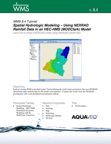
WMS TutorialsSpatial Hydrologic Modeling – Using NEXRAD Rainfall Data in an HEC-HMS (MODClark) Model10. In the Convert Grids dialog, make sure the Convert inches to millimetersoption is toggled off (Figure 6-3).Figure 6-3: Convert Grids dialog11. Click on the Browse buttonand browse to the folder/filespatial\HMS\NEXRAD\radarrain.dss (use the folder where you havesaved the data used in this tutorial) and click Save. It is advisable to select aname that is different than the HMS file you will later save (selecting adifferent name will separate the gridded precipitation dss file from theproject dss file and help keep your files organized).12. Set the Starting date to 7/25/2007 and the Starting time to 6:00 PM. Makesure the time interval is set to 1 hour (60 min) and click OK.13. After selecting OK, it will take some time to read and process theprecipitation files and save the gridded DSS file. You will see a few blackDOS windows popping up at the end of the process.For more information on how this process ishttp://www.xmswiki.com/index.php?title WMS:Radar Rainfallcarriedout,see14. As soon as the saving process completes, a summary file will open upshowing the date/time and rainfall depth at each time interval (Figure 6-4).Minimize this file; you will need it later on.Page 7 of 10 Aquaveo 2011

WMS TutorialsSpatial Hydrologic Modeling – Using NEXRAD Rainfall Data in an HEC-HMS (MODClark) ModelFigure 6-4: NEXRAD Radar Data summary report15. Click OK.7Visualizing Meteorological DataBefore continuing, let us visualize the gridded rainfall data.1. Select Close to close the wizard dialog.2. Turn off the display of soil type and land use coverages as well as the GISlayers by un-checking them in the data tree. This will help you zoom intothe watershed area for better visualization.3. Right click on Rainfall Cumulative on the data tree under 2D Grid Dataand select Contour Options Select Color Fill for the Contour Method.Click OK.4. Click on Rainfall Cumulative on the data tree under 2D Grid Data to makesure that it is active.5. Select the first time step in the properties window and with the down arrowkey on your keyboard, step through the time steps to see how theprecipitation varies.There are two rainfall datasets, one is incremental and the other is cumulative. You maychoose to view the incremental rainfall data set in the same way you viewed thecumulative data set. You may choose either dataset for creating the film loop.select Data Film Loop Specify the folder6. In the 2D Grid Modulewhere you want to have the animation saved, toggle off the option toExport to KMZ (Google Earth) and click Next.7. Under the option to Write to AVI file, make sure Rainfall Cumulative ischecked and that the option to write to a KMZ file is turned off for allPage 8 of 10 Aquaveo 2011

WMS TutorialsSpatial Hydrologic Modeling – Using NEXRAD Rainfall Data in an HEC-HMS (MODClark) Modeldatasets. Turn off the option to Write the 2D Scattered Dataset to a KMZFile.8. Click Next9. Click FinishWMS may take a few moments to create and save the animation file. The animation willstart playing as soon as the saving process is complete. Try to visualize how rainfall ischanging over the watershed over time. Let us now continue working with the model.8Saving the Model1. Open the Hydrologic Modeling Wizard dialog again by clicking thebutton.2. Click Clean Up Model on the left side of the dialog.3. Click on the Clean Up Model button. This button runs the operations thatare toggled on.4. Click OK to accept the default values for stream redistribution.5. In the model checker, fix any errors that may be listed, then click Done toclose the model checker.6. Click Close to close the modeling wizard dialog.7. Switch to the Hydrologic Modeling ModuleSave HMS file.and select HEC-HMS 8. Save the HMS file as spatial\ HMS\NEXRAD\wmsexport.hms.9Running the ModelWe have successfully created an HMS MODClark file for the Park City Watershed. Nowwe will work inside the HMS interface.1. Minimize the WMS window and open HEC-HMS 3.1 or later.2. Select File Open. Browse and open \spatial\HMS\NEXRAD\wmsexport.hms. If you do not have the .hms file saved properly, you mayopen it from \spatial\HMS\NEXRAD\finished \wmsexport.hms.3. Run the model (sometimes you must run the model twice for the results tobe active).4. View the results.10Using Rainfall Hyetograph and Running the Model Again1. Return to WMS.Page 9 of 10 Aquaveo 2011