Transcription
A33Reservoir Management Using Two-stageOptimization with Streamline SimulationT. Wen* (Stanford University), M.R. Thiele (Streamsim Technologies/Stanford University), D. Echeverría Ciaurri (IBM Thomas J. WatsonResearch Center), K. Aziz (Stanford University) & Y. Ye (StanfordUniversity)SUMMARYWaterflooding is a common secondary oil recovery process. Performance of waterfloods in mature fieldswith a significant number of wells can be improved with minimal infrastructure investment by optimizinginjection/production rates of individual wells. However, a major bottleneck in the optimization frameworkis the large number of reservoir flow simulations often required. In this work we propose a new methodbased on streamline-derived information that significantly reduces these computational costs in addition tomaking use of the computational efficiency of streamline simulation itself. We seek to maximize the longterm net present value of a waterflood by determining optimal individual well rates, given an expectedalbeit uncertain oil price and a total fluid injection volume. We approach the optimization problem bydecomposing it into two stages which can be implemented in a computationally efficient manner. The twostage streamline-based optimization approach can be an effective technique when applied to reservoirswith a large number of wells in need of an efficient waterflooding strategy over a 5 to 15 year period.ECMOR XIII – 13th European Conference on the Mathematics of Oil RecoveryBiarritz, France, 10-13 September 2012
IntroductionWaterflooding is a common secondary oil recovery process in which water is injected into an oil bearingreservoir using strategically placed injectors so as to maintain pressure and sweep oil to adjacent production wells. However, the efficiency of a waterflood will depend on a number of factors such as thedifferences in fluid properties, the spatial distribution of rock properties such as permeability, porosityand rock type, as well as the injection/production rates imposed at the wells.Many waterfloods are considered ’brown fields’ meaning that production has been occurring for manyyears ( 10), oil is produced in conjunction with large volumes of water ( 75%), and the total numberof wells is generally high ( 100). However, despite the high water production, a significant amount ofby-passed oil usually remains in such floods because they have generally been operated at sub-optimalconditions for many years. As a result, oil production may be enhanced significantly with minimal infrastructure investment simply by changing injection/production rates of individual wells currently operating. Additional enhancements, such as re-completions, side-tracks, and new infill wells can increaserecovery further, although these interventions tend to be more capital intensive. The effort to improve theperformance of brown fields has lead to closed-loop reservoir management strategies in which the inherent nonlinearity of the recovery processes is addressed formally by means of optimization approaches(Jansen et al. (2009); Wang et al. (2009); Sarma et al. (2005)).In the context of closed-loop reservoir management, production optimization is often formulated assuming a given geological scenario and recovery mechanism (waterflood, CO2 -flooding, etc.) The goal is tomaximize/minimize an objective function (e.g. cumulative oil production, NPV, total water production)under a set of physical constraints (e.g. available water supply, individual well production/injection capabilities), and economic constraints (e.g. oil price, tax regimes). The most immediate control variablesare injection/production well rates as these represent how floods are actually managed/implemented.Setting optimal well target rates is the focus of our work.The main challenge in formulating the production optimization problem is to account for the nonlinearity inherent in the recovery process. Nonlinear optimization methods can be roughly divided into twomain categories. The first family of methods refers to those procedures that use derivative informationdetermined from the cost function and/or constraints. In general, gradient-based techniques (Nocedaland Wright (2006); Luenberger and Ye (2008)) converge to local optima. Usually these solutions maynot be acceptable from a cost function perspective if important nonlinearities are present in the optimization. The most straightforward approach for computing derivatives is by means of finite-differenceapproximations. In this case, the estimation of the gradients requires a number of cost function evaluations on the order of the number of control variables. Since the evaluation of the cost function usuallyinvolves complex and time-demanding simulations, approximating derivatives numerically is expensive.Additionally, a common issue in finite-difference approximations is finding the proper perturbation sizein the numerical gradient used (large perturbation sizes may yield inaccurate derivatives, and small perturbation sizes may cause numerical issues due to the resolution of the simulator). In some cases gradientinformation can be extracted from the simulator in an efficient manner; adjoint-based methods (Sarmaet al. (2006); Brouwer and Jansen (2002)) are a very well-known technique for rapid computation ofderivatives. However, these methods require detailed knowledge of and access to the source code of thesimulator used, and that can be a limitation in practice.The second family of optimization techniques comprises procedures that do not require gradient information. Derivative-free algorithms (Kolda et al. (2003); Conn et al. (2009); Kramer et al. (2011); Echeverría Ciaurri et al. (2011)) can be subdivided into local optimization methods and global search schemes.The first type of methods have computational costs similar to gradient-based methods, but are somewhatmore robust from a theoretical perspective (for example, the issue of the perturbation size for the finitedifferences is solved in many derivative-free algorithms). Although (most) local derivative-free meth-ECMOR XIII – 13th European Conference on the Mathematics of Oil RecoveryBiarritz, France, 10-13 September 2012
ods guarantee convergence only to local optima, many of these techniques incorporate some amountof global exploration that may avoid being trapped in solutions that are not satisfactory from a costfunction point of view. Examples of derivative-free optimization methods that rely on local search areGeneralized Pattern Search (GPS; Audet and Dennis Jr (2002)), Mesh Adaptive Direct Search (MADS;Audet and Dennis Jr (2006)), and Hooke-Jeeves Direct Search (HJDS; Hooke and Jeeves (1961)). Inglobal search schemes the optimization space is analyzed much more thoroughly than in local methods,but at the expense of a larger computational cost. It is important to note that in the majority of practicaloptimization problems the global optimum cannot be obtained (the curse of dimensionality makes thisenterprise infeasible as soon as the number of optimization variables is larger than a few tens, somethingthat happens very often in real-life situations). Many global search algorithms resort to stochastic heuristics to prevent the whole process from terminating prematurely at a solution with a cost function that isunacceptable. These heuristics are rarely supported by formal optimization theory, and this is translatedin algorithmic parameters that are difficult to tune (as is the case of the population size in genetic algorithms). As a consequence, the use of global search methods requires a significant amount of experience,and in some cases the performance of these methods can be rather unpredictable. Examples of globalsearch procedures are genetic algorithms (GAs; Goldberg (1989)), particle swarm optimization (PSO;Kennedy and Eberhart (1995)), and differential evolution (DE; Storn and Price (1997)). We note thatderivative-free optimization methods can be easily implemented in a distributed manner, and thereforebe fairly efficient in terms of elapsed clock time (if a parallel computing environment is available) .In our work, we seek to maximize the long-term (generally 5 to 15 years) NPV of a waterflood, given acumulative target limit of the total field injection volume in conjunction with an uncertain oil price. Thegoal is to determine (near) optimal individual well rates that are sustainable (subject to constraints, suchas gradual changes over time as well as globally maximum/minimum total fluid rate handling capacities). To reduce the computational costs, we make use of streamline-derived information to drive thewell rate changes while also taking advantage of the computational efficiency of streamline simulationitself, which is generally well-suited for modeling waterfloods. We additionally speed-up the entire optimization process by decomposing the optimization problem into two stages: short-term and long-term.In the short-term stage, the NPV is maximized by setting optimal well controls (injected/produced totalfluid well rates) subject to a fixed total volume injection target. In the long-term stage, the sequence oftotal volume injection targets of all short-term periods is iteratively updated according to the expectedoil price and the long-term reservoir behavior approximated by an exponential decline model.This two-stage decomposition is computationally efficient because the optimizations for the short-termperiods use local information, that can be interpreted as approximate derivatives, derived from the connectivity information provided by the streamlines which require only a single streamline simulation(and thus, the computational cost associated to the estimation of the approximate derivatives becomesindependent of the total number of wells). The outer loop (long-term) optimization is accelerated byapproximating the long-term reservoir behavior through an analytical (exponential) decline model. Theapproach is validated on two waterflood scenarios where we find a significant speedup compared to othersingle-stage optimization methods, for the same quality of the solution.The paper is organized as follows. In the next section, we define the short-term optimization problemand show how streamline-based simulation can be used within the solution approach. In the sectionon long-term reservoir management, we define the long-term optimization problem, and explain howthe exponential decline model can be combined together with streamline simulation to approximate aglobal, long-term optimal solution. After that, we include a section where we present example caseswith practical relevance and compare our approach with a single-stage direct search (derivative-free)method. We end the paper with some discussion and conclusion.ECMOR XIII – 13th European Conference on the Mathematics of Oil RecoveryBiarritz, France, 10-13 September 2012
Short-Term Reservoir ManagementIn a short-term (less than one year) reservoir management problem, we are interested in finding optimalwell control settings so as to maximize profit but without accounting for fluctuations and discounting inthe oil price as we assume the price change and discount factor is small in a short-term period. Before weintroduce the mathematical formulation of the short-term reservoir management problem, we introducethe notation used in this section.The numbers of producers and injectors are denoted by NP and NI , respectively. qPo j and qPw j denote the oil and water rates at the jth producer, and the total fluid rates on the ith injector and the jth producer are respectively represented by qIw i and qPf . Note that qIw , qPfjare the vectors of the flow rates of all injectors/producers, which are the optimization variables. And qPois the vector of oil rates of all producers. ro is the oil price per unit volume of oil, and cwi and cwp arethe costs for water injection and for water production per unit volume of water, respectively. t is thelength of the short-term optimization period.We define the short-term optimization problem as follows: PPImaximizero Nj 1qPo j cwp Nj 1qPw j cwi Ni 1qIw i t,PqIw ,qfsubject to F qIw , qPf ; x qPo , NINPIq u, i 1 w i j 1 qPf Cu,j PPPqo j qw j q f j , j 1, 2, . . . , NP , LiI qIw i UiI , i 1, 2, . . . , NI , LPj qPf j U jP , j 1, 2, . . . , NP .(1a)(1b)(1c)(1d)(1e)(1f)In the objective function (1a), we define profit as the revenue from oil production subtracted by the costfor water injection and for the disposal/separation of produced water. We reiterate that the optimizationvariables are the total fluid rates on injectors and producers, i.e. qIw and qPf . The relation between theoil produced at each well and the fluid rate controls (given the current reservoir state x) is expressedin Equation (1b). The function F is generally complex and highly nonlinear, and must be evaluatedwith a numerical reservoir simulator. In our work, F is based on a streamline simulator (StreamsimTechnologies (2012)) that in the examples studied here yields significant speedup with respect to finitedifference/finite-volume simulation approaches. The constraint (1c) refers to a total injection volume,here u and C are parameters given by the user and they represent the field total injection target and thevoidage replacement ratio. As indicated above, the short-term optimization problem will be the basicbuilding block used to solve the long-term optimization problem. Note that the short-term optimizationproblem is stated for a relatively short production time frame, and that the well flow rates are assumedconstant during the period. The long-term optimization involves time explicitly, and it is essentiallya loop over short-term optimization with different values of total field injection u. We will see in thesection on long-term reservoir management that the sequence of u is selected so that the cumulatedlong-term profit determined by a fast-to-evaluate modified exponential decline model is maximized (thisstrategy takes into account the variation in the oil price, and avoids, in particular, low/high oil productionduring periods where the price is expected to be high/low). The constraint (1d) restricts that, at anyproducer, the sum of the oil flow rate and the water flow rate has to be equal to the total fluid rate. Thefluid rate targets of each well are required to stay within a minimum/maximum range (see (1e) and (1f)).In this work we opt for solving the optimization problem (1a)-(1f) using a derivative-free approach, motivated by the following two facts: first, the simulator available does not include methods for determiningderivatives rapidly (e.g. adjoint-based procedures); second, as indicated earlier, numerical derivativesapproximated by finite-differences present the problematic issue of finding the right perturbation size.ECMOR XIII – 13th European Conference on the Mathematics of Oil RecoveryBiarritz, France, 10-13 September 2012
Since the computational cost associated to each evaluation of F dominates all other calculations in theoptimization problem, the algorithm considered for solving this problem should make economic use ofthe function F .Here we propose to exploit the physical interpretation of streamlines to reduce the number of evaluationsof the function F in the complete optimization process. In essence, by means of streamline simulationwe will be able to (roughly) approximate the gradient of the cost function using only one reservoirsimulation. This is a significant reduction with respect to, for example, the approximation performedvia finite differences, where the number of cost function evaluations is on the order of optimizationvariables (and in this case equal to the number of wells). Although the gradient estimation obtainedusing streamlines in general will not be as good as the one determined with finite differences, in manycases (as is illustrated in later section) it will be good enough to iteratively provide improvement in theoptimization, and to eventually reach the proximity of a satisfactory local solution in an efficient manner.We introduce the general concept of streamline simulation next.Streamline Simulation and Flux Pattern MapStreamline simulation is an alternative reservoir simulation approach to the more widely used finitedifference/finite-volume approaches (Aziz and Settari (1979)). Although streamlines have been in thepetroleum literature since the early days of Muskat and Wyckoff (1937), modern streamline simulationemerged in the early 90s and distinguishes itself by six key ideas: 1) tracing 3D streamlines using theconcept of time-of-flight (TOF) rather than arc length; (2) expressing the mass conservation equationsin terms of TOF; (3) periodic updating of the streamlines in time; (4) solving the transport problemsnumerically along the streamlines rather than analytically; (5) accounting for gravity effects; and (6)extension to compressible flow (Thiele et al. (2010)). Because streamlines connect injectors and producers, streamline simulation has been successful at modeling floods that are dominated by the relativelocation and strength of injectors and producers and by the connectivity inherent in the underlying geological model. In such cases, streamline simulation is efficient in supplying engineering data that allowsa more physically-based optimization approach (Batycky et al. (1997); Thiele (2005)). The efficiencyof streamline simulation has led to its use for reservoir management (Lolomari et al. (2000); Thiele andBatycky (2006); Batycky et al. (2006)) and history matching (Wang and Kovscek (2000); Milliken et al.(2001); Caers et al. (2002)). Figure 1 displays an instantaneous streamline map for a two-dimensionalcase with three injectors and five producers.A key difference between streamline simulation and other simulation approaches is that the two/threedimensional transport calculations are decomposed into a series of one-dimensional problems alongstreamlines, and this generally leads to significant speedups and is advantageous in the context of anoptimization approach. However, in this work we focus on the additional information supplied by thestreamlines to help build a local, linear surrogate model to approximate the necessary derivatives to drivethe optimization approach. Specifically, we make use of flux pattern (FP) maps1 (Thiele and Batycky(2006)), which are simplified views of the injector/producer pairs captured by the streamlines (Figure2). As with streamlines, the FP maps represent the connectivity between injectors and producers atthat instant in time. Here for each connection in a FP map we make use of four sets of parametersidentifying ratios of injected/produced fluids from this connection. This is because each connectionsimply represents the sum of the volume fluxes (in and out) of all the streamlines associated with thatinjector-producer pair. Thus, for each connection we can define: PIPqqPffqw i jqo jijijiRIi Pj I , RPj Ii , EIi Pj , CIi Pj I,(qw )i(qw )i jqPfqPfj1 ThejiFPmap is protected by US patent #6,519,531 and used here with permission.ECMOR XIII – 13th European Conference on the Mathematics of Oil RecoveryBiarritz, France, 10-13 September 2012
Figure 1 Instantaneous streamline map obtained from a streamline simulation for a two-dimensionalheterogeneous case with three injectors and five producers. The streamlines are colored by injector/producer bundles.where qIw Pfand qPo ji are respecjiij jitively the rates of total fluid and oil at producer Pj due to injector Ii .RIi Pj and RPj Ii are volume ratios of total fluids injected/produced between well pairs with respect tothe injected/produced fluids at the wells. These ratios are equivalent to the well-known well allocationfactors, except that now they are determined using streamlines (Thiele and Batycky (2006); BatyckyPIRIi Pj 1 (and Ni 1RPj Ii 1)et al. (2006)), and therefore change in time. We note that in general Nj 1since not necessarily all the water injected at Ii can be associated with a producer (and not all the fluidproduced at Pj can be associated with an injector). The injection efficiency of an injector-producerpair EIi Pj is equivalent to an oil cut except that it is a ratio of oil produced to water injected. It isnoteworthy that the oil cut of an injector-producer pair EIi Pj is something that is generally not knownin standard simulation approaches. Finally, for compressible fluids CIi Pj is the volume ratio of totalfluids (in and out) associated with an injector-producer pair, and represents the well-known voidagereplacement ratio. Again, having this information for each injector-producer pair is unusual. For anyreservoir the parameter set{RIi Pj , RPj Ii , EIi Pj ,CIi Pj : i 1, 2, . . . , NI , j 1, 2, . . . , NP }describes uniquely the FP map at any instant in time and therefore the connectivity among injectors andproducers in the field. In Figure 2 we show the ratios associated to injector I4 for the flux pattern mapderived from Figure 1Flow Problem Linearization and Optimization ProcessThe central premise of our work is that we can use the FP map to ‘linearize’ the flow problem betweentime steps, and thus estimate derivatives using a single (streamline) simulation. Although the FP mapdepends on the well control setting (i.e. qIw , qPf ), we assume that it does not change significantly in amodest small neighborhood around a given control setting. In this work this neighborhood of (qIw , qPf )will be referred as the trust region and will be denoted by N (qIw , qPf ). The assumption above is partiallyECMOR XIII – 13th European Conference on the Mathematics of Oil RecoveryBiarritz, France, 10-13 September 2012
Figure 2 The left figure is the flux pattern map derived from the streamline map in Figure 1. The rightfigure shows the connections associated with injector I4 and related parameters.justified by the fact that a) in real fields rate changes for management purposes are usually done in smallincrements, and b) geological connectivity tends to dampen changes in streamline configuration due toPPsmall rate changes. As a result, we assume that oil and water production rates qo j and qw j may be reasonably represented as a linear function of water injection rates qIw i using the FP map: IIqIw i RIi Pj CIi Pj EIi Pj ,qPo ji Ni 1qPo j Ni 1(2a) IIqPw j Ni 1qPw ji Ni 1qIw i RIi Pj CIi Pj (1 EIi Pj ).(2b) PThe relation above allows us to linearize the nonlinear constraint F qIw , qPf ; x qo in the originalIPshort-term problem. We reiterate that for a given set of controls qw 0 and qf 0 for which the FP map is determined, the linearization is assumed to be valid only in the neighborhood N qIw 0 , qPf 0 .Also notice that the linearization implies the assumption that the perturbation of the control settings onproducers is determined by the perturbation of the control settings on injectors under the assumption ofa fixed FP map (since the fluid rate of a producer is determined by the injection rates of injectors; see(2a) and (2b)). We can also generate another linearization based on the same FP map determined byqIw 0 and qPf 0 as follows: IIqPo j Ni 1qPo ji Ni 1qPf RPj Ii EIi Pj ,(3a)j IIqPw ji Ni 1qPf RPj Ii (1 EIi Pj ).(3b)qPw j Ni 1jFrom the point of view of physics, both linearized forms are reasonable, since the principal assumptionis that oil and water are being produced by a displacement process rather than by expansion. Fromthe point of viewof mathematical optimization, both linearizations provide (partial) local information around ( qIw 0 , qPf 0 ). The alternating method is a general approach for this situation (Boyd et al.(2011)); it alternately uses a part of local information to search for the next trial step. We implement ourmethod in this alternating manner, i.e. at consecutive trial control settings, we use different linearizationsto approximate derivatives.IPThe linearization function (either of the two forms above) is denoted here by LF (qw , qf ) and by conPPIPstruction it satisfies qw 0 , qo 0 LF qw 0 , qf 0 . Thus, in the neighborhood of a current trialECMOR XIII – 13th European Conference on the Mathematics of Oil RecoveryBiarritz, France, 10-13 September 2012
control setting given by qIw 0 and qPf 0 , the short-term optimization problem (1a)-(1f) can be replacedby the following linear programming problem: IPP(4a)qIw i t,qPw j cwi Ni 1maximizeqPo j cwp Nj 1ro Nj 1qIw ,qPf N ((qIw )0 ,(qPf )0 ) subject toqPw , qPo LF qIw , qPf ,(4b) NIP(4c)qPf Cu,qIw i u, Nj 1 i 1j qPo j qPw j qPf j ,j 1, 2, . . . , NP ,(4d) LiI qIw i UiI , i 1, 2, . . . , NI ,(4e) PPPL j q f j U j , j 1, 2, . . . , NP .(4f)The solution for (4a)-(4f) is sought only in the trust region. As a consequence, in order to estimate asolution for (1a)-(1f) by means of an approach based on FP maps, it appears that a number of iterationsthat involve problems similar to (4a)-(4f) are needed. To solve the convex optimization problem (4a)(4f), we use CVX, a package for specifying and solving convex programs (Grant and Boyd (2011)).We reiterate here that our method alternately uses linearization forms (2a)-(2b) and (3a)-(3b) along theiteration steps.In each iteration step, the solution to (4a)-(4f) is the next trial control setting in the next iteration step.Note that the linearization is constructed with only one streamline simulation, hence the number ofsimulations required for one optimization step is one, which is much less than what is required for otherderivative-free methods (on the order of the number of optimization variables NI NP ). Therefore, thestreamline-based method presented here can be expected to be more efficient than many derivative-freemethods assuming the problem at hand can be reasonably represented by streamline simulation.The radius of the trust region (defined by the Euclidean norm here) is modified during optimization toreflect the accuracy of the linearized model. If the linearization LF approximates the real model Fwell in the trust region, then the radius of the trust region can be increased. On the other hand, if theapproximation is not acceptable in the complete trust region, then the radius of the trust region has to bereduced. Consistent with trust-region theory (Conn et al. (2000)), given the control setting qIw 0 and qPf 0 used to determine the FP map, we estimate the accuracy of the approximation at the next trial control setting qIw 1 , qPf 1 N qIw 0 , qPf 0 by J LF qIw 0 , qPf 0 J LF qIw 1 , qPf 1 θ (5)J F (qIw )0 , qPf 0 J F (qIw )1 , qPf 1where J denotes the profit function of oil/water production rates (Equation 1a and 4a). If θ is close toone, it indicates that the approximation is acceptable, otherwise it needs to be revised. It is important tonote, as described in the description of the algorithm below, that the computation of θ does not requireany additional streamline simulation or evaluation of the linearized model.The short-term optimization method proposed in this work is as follows: 1. Set an initial guess of the optimal control setting qIw 0 and qPf 0 , and of the initial radius r ofthe trust region2 . 2. Run a streamline simulation with qIw 0 and qPf 0 , and determine the FP map.2 We use a trust region radius smaller but on the same order of the radius of the original feasible region of problem (1a)-(1f)asthe initial radius.ECMOR XIII – 13th European Conference on the Mathematics of Oil RecoveryBiarritz, France, 10-13 September 2012
3. Use the FP map information from qIw 0 and qPf 0 to set-up the approximation and linearized problem (4a)-(4f). Solve for qIw 1 and qPf 1 . 4. Run streamline simulation with qIw 1 and qPf 1 , determine the FP map, and determine θ fromEquation (5). 5. If θ 0.5, update qIw 0 and qPf 0 as qIw 1 and qPf 1 .6. If 0.5 θ 2, increase r by 1.5 times. If θ 4 or θ 0.25, decrease r by 1/3.7. If the change in the objective function value is less than a user-defined tolerance, return qIw qPf 0 as solution, otherwise go to 2. 0andThe trust-region approach implemented in this work does not fully follow the basic trust-region optimizationmethod(see e.g. Conn et al. (2000)) because the gradient of the linearized model LF at IP( qw 0 , qf 0 ) does not coincide with the gradient of the function F at that point (the surrogate in thebasic algorithm in Conn et al. (2000)). However, based on the fact that the FP map can be used in general as an acceptable approximation of streamline simulation for short-term production computations,we can expect that both gradients provide similar information, and that the trust-region algorithm presented here yields an effective and efficient short-term optimization approach (as can be seen later in thecase examples reported in this paper).Long-Term Reservoir ManagementThe long-term reservoir management problem seeks a sequence of control settings during a long timehorizon (typically more than 5 years) which maximizes some performance metric such as the expectednet present value (NPV) (see e.g. van Essen et al. (2011)). This problem is of great importance in maturefields where a sustainable operation or strategy is a must to guarantee a high production level if oil pricerises in future. In this work, the performance metric is NPV, defined as a weighted sum of the profit ineach period:!NINPNTNP wpI k(6)NPV rko qPo j,k ck qPw j,k cwik qw i,k tk (1 d) ,k 1j 1j 1i 1where d is the discount factor, and all the time-varying quantities have the subindex ’k’ with respect tothose that were considered fixed in the short-term NPV definition used in Equation (1a).In the scenario where the field production efficiency decreases to a low level and the expected oil pricedoes not inc
Reservoir Management Using Two-stage Optimization with Streamline Simulation T. Wen* (Stanford University), M.R. Thiele (Streamsim Technologies/ Stanford University), D. Echeverría Ciaurri (IBM Thomas J. Watson Research Center), K. Aziz (Stanford University) & Y. Ye (Stanford University) SUMMARY Waterflooding is a common secondary oil recovery .