Transcription
Convex Optimization — Boyd & Vandenberghe1. Introduction mathematical optimization least-squares and linear programming convex optimization example course goals and topics nonlinear optimization brief history of convex optimization1–1
Mathematical optimization(mathematical) optimization problemminimize f0(x)subject to fi(x) bi,i 1, . . . , m x (x1, . . . , xn): optimization variables f0 : Rn R: objective function fi : Rn R, i 1, . . . , m: constraint functionsoptimal solution x has smallest value of f0 among all vectors thatsatisfy the constraintsIntroduction1–2
Examplesportfolio optimization variables: amounts invested in different assets constraints: budget, max./min. investment per asset, minimum return objective: overall risk or return variancedevice sizing in electronic circuits variables: device widths and lengths constraints: manufacturing limits, timing requirements, maximum area objective: power consumptiondata fitting variables: model parameters constraints: prior information, parameter limits objective: measure of misfit or prediction errorIntroduction1–3
Solving optimization problemsgeneral optimization problem very difficult to solve methods involve some compromise, e.g., very long computation time, ornot always finding the solutionexceptions: certain problem classes can be solved efficiently and reliably least-squares problems linear programming problems convex optimization problemsIntroduction1–4
Least-squaresminimize kAx bk22solving least-squares problems analytical solution: x (AT A) 1AT b reliable and efficient algorithms and software computation time proportional to n2k (A Rk n); less if structured a mature technologyusing least-squares least-squares problems are easy to recognize a few standard techniques increase flexibility (e.g., including weights,adding regularization terms)Introduction1–5
Linear programmingminimize cT xsubject to aTi x bi,i 1, . . . , msolving linear programs no analytical formula for solution reliable and efficient algorithms and software computation time proportional to n2m if m n; less with structure a mature technologyusing linear programming not as easy to recognize as least-squares problems a few standard tricks used to convert problems into linear programs(e.g., problems involving ℓ1- or ℓ -norms, piecewise-linear functions)Introduction1–6
Convex optimization problemminimize f0(x)subject to fi(x) bi,i 1, . . . , m objective and constraint functions are convex:fi(αx βy) αfi(x) βfi(y)if α β 1, α 0, β 0 includes least-squares problems and linear programs as special casesIntroduction1–7
solving convex optimization problems no analytical solution reliable and efficient algorithms computation time (roughly) proportional to max{n3, n2m, F }, where Fis cost of evaluating fi’s and their first and second derivatives almost a technologyusing convex optimization often difficult to recognize many tricks for transforming problems into convex form surprisingly many problems can be solved via convex optimizationIntroduction1–8
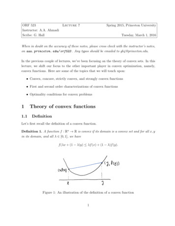
Examplem lamps illuminating n (small, flat) patcheslamp power pjrkjθkjillumination Ikintensity Ik at patch k depends linearly on lamp powers pj :Ik mXakj pj , 2max{cos θkj , 0}akj rkjj 1problem: achieve desired illumination Ides with bounded lamp powersminimize maxk 1,.,n log Ik log Ides subject to 0 pj pmax, j 1, . . . , mIntroduction1–9
how to solve?1. use uniform power: pj p, vary p2. use least-squares:minimizeround pj if pj pmax or pj 0Pn2(I I)kdesk 13. use weighted least-squares:PnPm22minimizek 1 (Ik Ides ) j 1 wj (pj pmax /2)iteratively adjust weights wj until 0 pj pmax4. use linear programming:minimize maxk 1,.,n Ik Ides subject to 0 pj pmax, j 1, . . . , mwhich can be solved via linear programmingof course these are approximate (suboptimal) ‘solutions’Introduction1–10
5. use convex optimization: problem is equivalent tominimize f0(p) maxk 1,.,n h(Ik /Ides)subject to 0 pj pmax, j 1, . . . , mwith h(u) max{u, 1/u}5h(u)43210012u34f0 is convex because maximum of convex functions is convexexact solution obtained with effort modest factor least-squares effortIntroduction1–11
additional constraints: does adding 1 or 2 below complicate the problem?1. no more than half of total power is in any 10 lamps2. no more than half of the lamps are on (pj 0) answer: with (1), still easy to solve; with (2), extremely difficult moral: (untrained) intuition doesn’t always work; without the properbackground very easy problems can appear quite similar to very difficultproblemsIntroduction1–12
Course goals and topicsgoals1. recognize/formulate problems (such as the illumination problem) asconvex optimization problems2. develop code for problems of moderate size (1000 lamps, 5000 patches)3. characterize optimal solution (optimal power distribution), give limits ofperformance, etc.topics1. convex sets, functions, optimization problems2. examples and applications3. algorithmsIntroduction1–13
Nonlinear optimizationtraditional techniques for general nonconvex problems involve compromiseslocal optimization methods (nonlinear programming) find a point that minimizes f0 among feasible points near it fast, can handle large problems require initial guess provide no information about distance to (global) optimumglobal optimization methods find the (global) solution worst-case complexity grows exponentially with problem sizethese algorithms are often based on solving convex subproblemsIntroduction1–14
Brief history of convex optimizationtheory (convex analysis): ca1900–1970algorithms 1947: simplex algorithm for linear programming (Dantzig)1960s: early interior-point methods (Fiacco & McCormick, Dikin, . . . )1970s: ellipsoid method and other subgradient methods1980s: polynomial-time interior-point methods for linear programming(Karmarkar 1984) late 1980s–now: polynomial-time interior-point methods for nonlinearconvex optimization (Nesterov & Nemirovski 1994)applications before 1990: mostly in operations research; few in engineering since 1990: many new applications in engineering (control, signalprocessing, communications, circuit design, . . . ); new problem classes(semidefinite and second-order cone programming, robust optimization)Introduction1–15
Convex Optimization — Boyd & Vandenberghe2. Convex sets affine and convex sets some important examples operations that preserve convexity generalized inequalities separating and supporting hyperplanes dual cones and generalized inequalities2–1
Affine setline through x1, x2: all pointsx θx1 (1 θ)x2(θ R)x1θ 1.2θ 1θ 0.6x2θ 0θ 0.2affine set: contains the line through any two distinct points in the setexample: solution set of linear equations {x Ax b}(conversely, every affine set can be expressed as solution set of system oflinear equations)Convex sets2–2
Convex setline segment between x1 and x2: all pointsx θx1 (1 θ)x2with 0 θ 1convex set: contains line segment between any two points in the setx1, x2 C,0 θ 1 θx1 (1 θ)x2 Cexamples (one convex, two nonconvex sets)Convex sets2–3
Convex combination and convex hullconvex combination of x1,. . . , xk : any point x of the formx θ1 x1 θ2 x2 · · · θk xkwith θ1 · · · θk 1, θi 0convex hull conv S: set of all convex combinations of points in SConvex sets2–4
Convex coneconic (nonnegative) combination of x1 and x2: any point of the formx θ1 x1 θ2 x2with θ1 0, θ2 0x1x20convex cone: set that contains all conic combinations of points in the setConvex sets2–5
Hyperplanes and halfspaceshyperplane: set of the form {x aT x b} (a 6 0)ax0xaT x bhalfspace: set of the form {x aT x b} (a 6 0)ax0aT x baT x b a is the normal vector hyperplanes are affine and convex; halfspaces are convexConvex sets2–6
Euclidean balls and ellipsoids(Euclidean) ball with center xc and radius r:B(xc, r) {x kx xck2 r} {xc ru kuk2 1}ellipsoid: set of the form{x (x xc)T P 1(x xc) 1}with P Sn (i.e., P symmetric positive definite)xcother representation: {xc Au kuk2 1} with A square and nonsingularConvex sets2–7
Norm balls and norm conesnorm: a function k · k that satisfies kxk 0; kxk 0 if and only if x 0 ktxk t kxk for t R kx yk kxk kyknotation: k · k is general (unspecified) norm; k · ksymb is particular normnorm ball with center xc and radius r: {x kx xck r}1Euclidean norm cone is called secondorder cone0.5tnorm cone: {(x, t) kxk t}0110x2 1 10x1norm balls and cones are convexConvex sets2–8
Polyhedrasolution set of finitely many linear inequalities and equalitiesAx b,Cx d(A Rm n, C Rp n, is componentwise inequality)a1a2Pa5a3a4polyhedron is intersection of finite number of halfspaces and hyperplanesConvex sets2–9
Positive semidefinite conenotation: Sn is set of symmetric n n matrices Sn {X Sn X 0}: positive semidefinite n n matricesX Sn z T Xz 0 for all z Sn is a convex cone Sn {X Sn X 0}: positive definite n n matrices1x yy z S2 0.5zexample: 0110yConvex sets0.5 1 0x2–10
Operations that preserve convexitypractical methods for establishing convexity of a set C1. apply definitionx1, x2 C,0 θ 1 θx1 (1 θ)x2 C2. show that C is obtained from simple convex sets (hyperplanes,halfspaces, norm balls, . . . ) by operations that preserve convexity intersectionaffine functionsperspective functionlinear-fractional functionsConvex sets2–11
Intersectionthe intersection of (any number of) convex sets is convexexample:S {x Rm p(t) 1 for t π/3}where p(t) x1 cos t x2 cos 2t · · · xm cos mtfor m 2:210x2p(t)1 1S0 10Convex setsπ/3t2π/3π 2 2 1x01122–12
Affine functionsuppose f : Rn Rm is affine (f (x) Ax b with A Rm n, b Rm) the image of a convex set under f is convexS Rn convex f (S) {f (x) x S} convex the inverse image f 1(C) of a convex set under f is convexC Rm convex f 1(C) {x Rn f (x) C} convexexamples scaling, translation, projection solution set of linear matrix inequality {x x1A1 · · · xmAm B}(with Ai, B Sp) hyperbolic cone {x xT P x (cT x)2, cT x 0} (with P Sn )Convex sets2–13
Perspective and linear-fractional functionperspective function P : Rn 1 Rn:P (x, t) x/t,dom P {(x, t) t 0}images and inverse images of convex sets under perspective are convexlinear-fractional function f : Rn Rm:Ax b,f (x) Tc x ddom f {x cT x d 0}images and inverse images of convex sets under linear-fractional functionsare convexConvex sets2–14
example of a linear-fractional functionf (x) 1xx1 x2 10 1 1Convex sets1x2x21C0x110 1 1f (C)0x112–15
Generalized inequalitiesa convex cone K Rn is a proper cone if K is closed (contains its boundary) K is solid (has nonempty interior) K is pointed (contains no line)examples nonnegative orthant K Rn {x Rn xi 0, i 1, . . . , n} positive semidefinite cone K Sn nonnegative polynomials on [0, 1]:K {x Rn x1 x2t x3t2 · · · xntn 1 0 for t [0, 1]}Convex sets2–16
generalized inequality defined by a proper cone K:x K y y x K,x K y y x int Kexamples componentwise inequality (K Rn )x Rn y xi yi ,i 1, . . . , n matrix inequality (K Sn )X Sn Y Y X positive semidefinitethese two types are so common that we drop the subscript in Kproperties: many properties of K are similar to on R, e.g.,x K y,Convex setsu K v x u K y v2–17
Minimum and minimal elements K is not in general a linear ordering : we can have x 6 K y and y 6 K xx S is the minimum element of S with respect to K ify S x K yx S is a minimal element of S with respect to K ify S,y K x example (K R2 )x1 is the minimum element of S1x2 is a minimal element of S2x1Convex setsS1y xS2x22–18
Separating hyperplane theoremif C and D are nonempty disjoint convex sets, there exist a 6 0, b s.t.aT x b for x C,aT x b for x DaT x baT x bDCathe hyperplane {x aT x b} separates C and Dstrict separation requires additional assumptions (e.g., C is closed, D is asingleton)Convex sets2–19
Supporting hyperplane theoremsupporting hyperplane to set C at boundary point x0:{x aT x aT x0}where a 6 0 and aT x aT x0 for all x CaCx0supporting hyperplane theorem: if C is convex, then there exists asupporting hyperplane at every boundary point of CConvex sets2–20
Dual cones and generalized inequalitiesdual cone of a cone K:K {y y T x 0 for all x K}examples K Rn : K Rn K Sn : K Sn K {(x, t) kxk2 t}: K {(x, t) kxk2 t} K {(x, t) kxk1 t}: K {(x, t) kxk t}first three examples are self-dual conesdual cones of proper cones are proper, hence define generalized inequalities:y K 0Convex sets y T x 0 for all x K 02–21
Minimum and minimal elements via dual inequalitiesminimum element w.r.t. Kx is minimum element of S iff for allλ K 0, x is the unique minimizerof λT z over SSxminimal element w.r.t. K if x minimizes λT z over S for some λ K 0, then x is minimalλ1x1Sx2λ2 if x is a minimal element of a convex set S, then there exists a nonzeroλ K 0 such that x minimizes λT z over SConvex sets2–22
optimal production frontier different production methods use different amounts of resources x Rn production set P : resource vectors x for all possible production methods efficient (Pareto optimal) methods correspond to resource vectors xthat are minimal w.r.t. Rn fuelexample (n 2)x1, x2, x3 are efficient; x4, x5 are notPx1x2 x5 x4λx3laborConvex sets2–23
Convex Optimization — Boyd & Vandenberghe3. Convex functions basic properties and examples operations that preserve convexity the conjugate function quasiconvex functions log-concave and log-convex functions convexity with respect to generalized inequalities3–1
Definitionf : Rn R is convex if dom f is a convex set andf (θx (1 θ)y) θf (x) (1 θ)f (y)for all x, y dom f , 0 θ 1(y, f (y))(x, f (x)) f is concave if f is convex f is strictly convex if dom f is convex andf (θx (1 θ)y) θf (x) (1 θ)f (y)for x, y dom f , x 6 y, 0 θ 1Convex functions3–2
Examples on Rconvex: affine: ax b on R, for any a, b R exponential: eax, for any a R powers: xα on R , for α 1 or α 0 powers of absolute value: x p on R, for p 1 negative entropy: x log x on R concave: affine: ax b on R, for any a, b R powers: xα on R , for 0 α 1 logarithm: log x on R Convex functions3–3
Examples on Rn and Rm naffine functions are convex and concave; all norms are convexexamples on Rn affine function f (x) aT x bPn norms: kxkp ( i 1 xi p)1/p for p 1; kxk maxk xk examples on Rm n (m n matrices) affine functionf (X) tr(AT X) b nm XXAij Xij bi 1 j 1 spectral (maximum singular value) normf (X) kXk2 σmax(X) (λmax(X T X))1/2Convex functions3–4
Restriction of a convex function to a linef : Rn R is convex if and only if the function g : R R,g(t) f (x tv),dom g {t x tv dom f }is convex (in t) for any x dom f , v Rncan check convexity of f by checking convexity of functions of one variableexample. f : Sn R with f (X) log det X, dom f Sn g(t) log det(X tV ) log det X log det(I tX 1/2V X 1/2)nXlog(1 tλi) log det X i 1where λi are the eigenvalues of X 1/2V X 1/2g is concave in t (for any choice of X 0, V ); hence f is concaveConvex functions3–5
Extended-value extensionextended-value extension f of f isf (x) f (x),x dom f,f (x) ,x 6 dom foften simplifies notation; for example, the condition0 θ 1 f (θx (1 θ)y) θf (x) (1 θ)f (y)(as an inequality in R { }), means the same as the two conditions dom f is convex for x, y dom f ,0 θ 1Convex functions f (θx (1 θ)y) θf (x) (1 θ)f (y)3–6
First-order conditionf is differentiable if dom f is open and the gradient f (x) f (x) f (x) f (x),,., x1 x2 xn exists at each x dom f1st-order condition: differentiable f with convex domain is convex ifff (y) f (x) f (x)T (y x)for all x, y dom ff (y)f (x) f (x)T (y x)(x, f (x))first-order approximation of f is global underestimatorConvex functions3–7
Second-order conditionsf is twice differentiable if dom f is open and the Hessian 2f (x) Sn, 2f (x) f (x)ij , xi xj2i, j 1, . . . , n,exists at each x dom f2nd-order conditions: for twice differentiable f with convex domain f is convex if and only if 2f (x) 0for all x dom f if 2f (x) 0 for all x dom f , then f is strictly convexConvex functions3–8
Examplesquadratic function: f (x) (1/2)xT P x q T x r (with P Sn) 2f (x) P f (x) P x q,convex if P 0least-squares objective: f (x) kAx bk22 f (x) 2AT (Ax b), 2f (x) 2AT Aconvex (for any A)quadratic-over-linear: f (x, y) x2/yy x y x T 0f (x, y)2 2f (x, y) 3y 2102201convex for y 0Convex functionsy0 2x3–9
log-sum-exp: f (x) log 2f (x) 11T zPnk 1 exp xkdiag(z) is convex1Tzz(1T z)2(zk exp xk )to show 2f (x) 0, we must verify that v T 2f (x)v 0 for all v:T2v f (x)v since (Pk v k zk )2 (P(P2k zk vk )(2k zk vk )(geometric mean: f (x) (PPPzk ) ( k v k zk ) 2kP 0( k zk ) 2k zk )(from Cauchy-Schwarz inequality)Qnn1/nx)onRk is concavek 1(similar proof as for log-sum-exp)Convex functions3–10
Epigraph and sublevel setα-sublevel set of f : Rn R:Cα {x dom f f (x) α}sublevel sets of convex functions are convex (converse is false)epigraph of f : Rn R:epi f {(x, t) Rn 1 x dom f, f (x) t}epi fff is convex if and only if epi f is a convex setConvex functions3–11
Jensen’s inequalitybasic inequality: if f is convex, then for 0 θ 1,f (θx (1 θ)y) θf (x) (1 θ)f (y)extension: if f is convex, thenf (E z) E f (z)for any random variable zbasic inequality is special case with discrete distributionprob(z x) θ,Convex functionsprob(z y) 1 θ3–12
Operations that preserve convexitypractical methods for establishing convexity of a function1. verify definition (often simplified by restricting to a line)2. for twice differentiable functions, show 2f (x) 03. show that f is obtained from simple convex functions by operationsthat preserve convexity nonnegative weighted sumcomposition with affine functionpointwise maximum and supremumcompositionminimizationperspectiveConvex functions3–13
Positive weighted sum & composition with affine functionnonnegative multiple: αf is convex if f is convex, α 0sum: f1 f2 convex if f1, f2 convex (extends to infinite sums, integrals)composition with affine function: f (Ax b) is convex if f is convexexamples log barrier for linear inequalitiesf (x) mXi 1log(bi aTi x),dom f {x aTi x bi, i 1, . . . , m} (any) norm of affine function: f (x) kAx bkConvex functions3–14
Pointwise maximumif f1, . . . , fm are convex, then f (x) max{f1(x), . . . , fm(x)} is convexexamples piecewise-linear function: f (x) maxi 1,.,m(aTi x bi) is convex sum of r largest components of x Rn:f (x) x[1] x[2] · · · x[r]is convex (x[i] is ith largest component of x)proof:f (x) max{xi1 xi2 · · · xir 1 i1 i2 · · · ir n}Convex functions3–15
Pointwise supremumif f (x, y) is convex in x for each y A, theng(x) sup f (x, y)y Ais convexexamples support function of a set C: SC (x) supy C y T x is convex distance to farthest point in a set C:f (x) sup kx yky C maximum eigenvalue of symmetric matrix: for X Sn,λmax(X) sup y T Xykyk2 1Convex functions3–16
Composition with scalar functionscomposition of g : Rn R and h : R R:f (x) h(g(x))f is convex ifg convex, h convex, h̃ nondecreasingg concave, h convex, h̃ nonincreasing proof (for n 1, differentiable g, h)f ′′(x) h′′(g(x))g ′(x)2 h′(g(x))g ′′(x) note: monotonicity must hold for extended-value extension h̃examples exp g(x) is convex if g is convex 1/g(x) is convex if g is concave and positiveConvex functions3–17
Vector compositioncomposition of g : Rn Rk and h : Rk R:f (x) h(g(x)) h(g1(x), g2(x), . . . , gk (x))f is convex ifgi convex, h convex, h̃ nondecreasing in each argumentgi concave, h convex, h̃ nonincreasing in each argumentproof (for n 1, differentiable g, h)f ′′(x) g ′(x)T 2h(g(x))g ′(x) h(g(x))T g ′′(x)examplesPm i 1 log gi (x) is concave if gi are concave and positivePm log i 1 exp gi(x) is convex if gi are convexConvex functions3–18
Minimizationif f (x, y) is convex in (x, y) and C is a convex set, theng(x) inf f (x, y)y Cis convexexamples f (x, y) xT Ax 2xT By y T Cy with ABTBC 0,C 0minimizing over y gives g(x) inf y f (x, y) xT (A BC 1B T )xg is convex, hence Schur complement A BC 1B T 0 distance to a set: dist(x, S) inf y S kx yk is convex if S is convexConvex functions3–19
Perspectivethe perspective of a function f : Rn R is the function g : Rn R R,dom g {(x, t) x/t dom f, t 0}g(x, t) tf (x/t),g is convex if f is convexexamples f (x) xT x is convex; hence g(x, t) xT x/t is convex for t 0 negative logarithm f (x) log x is convex; hence relative entropyg(x, t) t log t t log x is convex on R2 if f is convex, thenTTg(x) (c x d)f (Ax b)/(c x d) is convex on {x cT x d 0, (Ax b)/(cT x d) dom f }Convex functions3–20
The conjugate functionthe conjugate of a function f isf (y) sup (y T x f (x))x dom ff (x)xyx(0, f (y)) f is convex (even if f is not) will be useful in chapter 5Convex functions3–21
examples negative logarithm f (x) log xf (y) sup(xy log x)x 0 1 log( y) y 0 otherwise strictly convex quadratic f (x) (1/2)xT Qx with Q Sn f (y) sup(y T x (1/2)xT Qx)x Convex functions1 T 1y Q y23–22
Quasiconvex functionsf : Rn R is quasiconvex if dom f is convex and the sublevel setsSα {x dom f f (x) α}are convex for all αβαabc f is quasiconcave if f is quasiconvex f is quasilinear if it is quasiconvex and quasiconcaveConvex functions3–23
Examples p x is quasiconvex on R ceil(x) inf{z Z z x} is quasilinear log x is quasilinear on R f (x1, x2) x1x2 is quasiconcave on R2 linear-fractional functionaT x b,f (x) Tc x ddom f {x cT x d 0}is quasilinear distance ratiokx ak2,f (x) kx bk2dom f {x kx ak2 kx bk2}is quasiconvexConvex functions3–24
internal rate of return cash flow x (x0, . . . , xn); xi is payment in period i (to us if xi 0) we assume x0 0 and x0 x1 · · · xn 0 present value of cash flow x, for interest rate r:PV(x, r) nX(1 r) ixii 0 internal rate of return is smallest interest rate for which PV(x, r) 0:IRR(x) inf{r 0 PV(x, r) 0}IRR is quasiconcave: superlevel set is intersection of open halfspacesIRR(x) RConvex functions nXi 0(1 r) ixi 0 for 0 r R3–25
Propertiesmodified Jensen inequality: for quasiconvex f0 θ 1 f (θx (1 θ)y) max{f (x), f (y)}first-order condition: differentiable f with cvx domain is quasiconvex ifff (y) f (x) f (x)T (y x) 0x f (x)sums of quasiconvex functions are not necessarily quasiconvexConvex functions3–26
Log-concave and log-convex functionsa positive function f is log-concave if log f is concave:f (θx (1 θ)y) f (x)θ f (y)1 θfor 0 θ 1f is log-convex if log f is convex powers: xa on R is log-convex for a 0, log-concave for a 0 many common probability densities are log-concave, e.g., normal:f (x) p1(2π)n det Σ1e 2 (x x̄)TΣ 1 (x x̄) cumulative Gaussian distribution function Φ is log-concaveZ x21Φ(x) e u /2 du2π Convex functions3–27
Properties of log-concave functions twice differentiable f with convex domain is log-concave if and only iff (x) 2f (x) f (x) f (x)Tfor all x dom f product of log-concave functions is log-concave sum of log-concave functions is not always log-concave integration: if f : Rn Rm R is log-concave, theng(x) Zf (x, y) dyis log-concave (not easy to show)Convex functions3–28
consequences of integration property convolution f g of log-concave functions f , g is log-concave(f g)(x) Zf (x y)g(y)dy if C Rn convex and y is a random variable with log-concave pdf thenf (x) prob(x y C)is log-concaveproof: write f (x) as integral of product of log-concave functionsf (x) Zg(x y)p(y) dy,g(u) 1 u C0 u 6 C,p is pdf of yConvex functions3–29
example: yield functionY (x) prob(x w S) x Rn: nominal parameter values for product w Rn: random variations of parameters in manufactured product S: set of acceptable valuesif S is convex and w has a log-concave pdf, then Y is log-concave yield regions {x Y (x) α} are convexConvex functions3–30
Convexity with respect to generalized inequalitiesf : Rn Rm is K-convex if dom f is convex andf (θx (1 θ)y) K θf (x) (1 θ)f (y)for x, y dom f , 0 θ 1example f : Sm Sm, f (X) X 2 is Sm -convexproof: for fixed z Rm, z T X 2z kXzk22 is convex in X, i.e.,z T (θX (1 θ)Y )2z θz T X 2z (1 θ)z T Y 2zfor X, Y Sm, 0 θ 1therefore (θX (1 θ)Y )2 θX 2 (1 θ)Y 2Convex functions3–31
Convex Optimization — Boyd & Vandenberghe4. Convex optimization problems optimization problem in standard form convex optimization problems quasiconvex optimization linear optimization quadratic optimization geometric programming generalized inequality constraints semidefinite programming vector optimization4–1
Optimization problem in standard formminimize f0(x)subject to fi(x) 0,hi(x) 0,i 1, . . . , mi 1, . . . , p x Rn is the optimization variable f0 : Rn R is the objective or cost function fi : Rn R, i 1, . . . , m, are the inequality constraint functions hi : Rn R are the equality constraint functionsoptimal value:p inf{f0(x) fi(x) 0, i 1, . . . , m, hi(x) 0, i 1, . . . , p} p if problem is infeasible (no x satisfies the constraints) p if problem is unbounded belowConvex optimization problems4–2
Optimal and locally optimal pointsx is feasible if x dom f0 and it satisfies the constraintsa feasible x is optimal if f0(x) p ; Xopt is the set of optimal pointsx is locally optimal if there is an R 0 such that x is optimal forminimize (over z) f0(z)subject tofi(z) 0, i 1, . . . , m,kz xk2 Rhi(z) 0,i 1, . . . , pexamples (with n 1, m p 0) f0(x) 1/x, dom f0 R : p 0, no optimal point f0(x) log x, dom f0 R : p f0(x) x log x, dom f0 R : p 1/e, x 1/e is optimal f0(x) x3 3x, p , local optimum at x 1Convex optimization problems4–3
Implicit constraintsthe standard form optimization problem has an implicit constraintx D m\i 0dom fi p\dom hi,i 1 we call D the domain of the problem the constraints fi(x) 0, hi(x) 0 are the explicit constraints a problem is unconstrained if it has no explicit constraints (m p 0)example:minimize f0(x) Pki 1 log(bi aTi x)is an unconstrained problem with implicit constraints aTi x biConvex optimization problems4–4
Feasibility problemfindxsubject to fi(x) 0,hi(x) 0,i 1, . . . , mi 1, . . . , pcan be considered a special case of the general problem with f0(x) 0:minimize 0subject to fi(x) 0,hi(x) 0,i 1, . . . , mi 1, . . . , p p 0 if constraints are feasible; any feasible x is optimal p if constraints are infeasibleConvex optimization problems4–5
Convex optimization problemstandard form convex optimization problemminimize f0(x)subject to fi(x) 0, i 1, . . . , maTi x bi, i 1, . . . , p f0, f1, . . . , fm are convex; equality constraints are affine problem is quasiconvex if f0 is quasiconvex (and f1, . . . , fm convex)often written asminimize f0(x)subject to fi(x) 0,Ax bi 1, . . . , mimportant property: feasible set of a convex optimization problem is convexConvex optimization problems4–6
exampleminimize f0(x) x21 x22subject to f1(x) x1/(1 x22) 0h1(x) (x1 x2)2 0 f0 is convex; feasible set {(x1, x2) x1 x2 0} is convex not a convex problem (according to our definition): f1 is not convex, h1is not affine equivalent (but not identical) to the convex problemminimize x21 x22subject to x1 0x1 x2 0Convex optimization problems4–7
Local and global optimaany locally optimal point of a convex problem is (globally) optimalproof: suppose x is locally optimal, but there exists a feasible y withf0(y) f0(x)x locally optimal means there is an R 0 such thatz feasible,kz xk2 R f0(z) f0(x)consider z θy (1 θ)x with θ R/(2ky xk2) ky xk2 R, so 0 θ 1/2 z is a convex combination of two feasible points, hence also feasible kz xk2 R/2 andf0(z) θf0(y) (1 θ)f0(x) f0(x)which contradicts our assumption that x is locally optimalConvex optimization problems4–8
Optimality criterion for differentiable f0x is optimal if and only if it is feasible and f0(x)T (y x) 0for all feasible y f0(x)Xxif nonzero, f0(x) defines a supporting hyperplane to feasible set X at xConvex optimization problems4–9
unconstrained problem: x is optimal if and only ifx dom f0, f0(x) 0 equality constrained problemminimize f0(x) subject to Ax bx is optimal if and only if there exists a ν such thatx dom f0, f0(x) AT ν 0Ax b, minimization over nonnegative orthantminimize f0(x) subject to x 0x is optimal if and only ifx dom f0,Convex optimization problemsx 0, f0(x)i 0 xi 0 f0(x)i 0 xi 04–10
Equivalent convex problemstwo problems are (informally) equivalent if the solution of one is readilyobtained from the solution of the other, and vice-versasome common transformations that pr
solving least-squares problems analytical solution: x (ata) 1atb reliable and efficient algorithms and software computation time proportional to n2k(a rk n); less if structured a mature technology using least-squares least-squares problems are easy to recognize a few standard techniques increase flexibility (e.g., including weights,