Transcription
Computational Fluid Dynamics Analysis of Air Flowand Temperature Distribution in BuildingsUndergraduate Honors ThesisPresented in Partial Fulfillment of the Requirements forGraduation with Distinction in Mechanical EngineeringByBradley S. HurakDefense Committee:Professor Sandip MazumderProfessor Yann Guezennec
AbstractEnergy consumption for the heating and cooling of residential buildings accounts for nearly halfof total use. Because the physical configuration of heating and cooling inlets and outlets is oftendetermined from historical practice or convenience rather than optimal performance, it stands toreason that there is an opportunity to gain effectiveness of these systems by applying engineeringprinciples to their design. In this study, a computational fluid dynamic analysis was performed toinvestigate the effect of the physical configuration of inlet and outlet vents on the temperature and flowpatterns inside a room modeled for simplicity as a two dimensional enclosure. It was determined thatfor use in both heating and cooling of a room, a low or floor located inlet vent coupled with an outletthat is positioned on the upper half of a wall yields the most desirable results in reaching, or nearlyreaching, comfort conditions in the shortest amount of time. However, if either heating or cooling isexpected to be the primary energy consumption, it may be advantageous to deviate from thisconfiguration.ii
AcknowledgementsI would like to thank everyone who has supported me throughout the course of this project. Iam appreciative for the help and patience of my advisor, Professor Sandip Mazumder. I have valued andlearned from the constructive criticism that Professor Yann Guezennec has offered throughout theclassroom sessions for this project. ESI Group is also acknowledged for providing lisences to theircommercial software, CFD-ACE . Finally, I am very grateful for the encouragement, support, and lovethat my parents have always given me.iii
Table of ContentsAbstract . iiAcknowledgements. iiiList of Figures . vList of Tables . vi123Introduction . 11.1Literature Survey. 11.2Objectives of Current Research . 2Methods . 32.1Two-dimensional Model Description . 32.2Three-dimensional Model Description . 42.3Parametric Study . 52.4Model Conditions . 62.4.1Hot Conditions . 62.4.2Cold Conditions . 7CFD Model. 83.1Flow Module . 83.1.1Mass Conservation Equation . 83.1.2Momentum Conservation Equations . 83.1.3Navier-Stokes Equations . 93.1.4Other Flow Properties . 103.2Heat Transfer Module . 113.2.14Thermal Boundaries . 113.3Turbulence Module . 153.4Three-dimensional Model Properties . 16Results . 174.1Flow Data . 174.2Temperature Data . 185Conclusions . 296Recommendations . 33Appendix A . 34Bibliography . 45iv
List of FiguresFigure 1: Two-dimensional model with inlets, outlets, and temperature probe. . 4Figure 2: Three-dimensional model with inlets and outlets. . 5Figure 3: Thermal resistance model of ceiling. . 13Figure 4: Thermal resistance model of side walls. . 14Figure 5: Thermal resistance model of floor. . 14Figure 6: Configuration 3-4, Cooling. . 18Figure 7: Monitor point temperature data, Inlet 2, Outlet 1. . 19Figure 8: Monitor point temperature data, Inlet 2, Outlet 2. . 20Figure 9: Monitor point temperature data, Inlet 2, Outlet 3. . 20Figure 10: Monitor point temperature data, Inlet 2, Outlet 4. . 21Figure 11: Monitor point temperature data, Inlet 2, Outlet 5. . 21Figure 12: Monitor point temperature data, Inlet 1, Outlet 2. . 23Figure 13: Monitor point temperature data, Inlet 2, Outlet 2. . 23Figure 14: Monitor point temperature data, Inlet 3, Outlet 2. . 24Figure 15: Monitor point temperature data, Inlet 4, Outlet 2. . 24Figure 16: Monitor point temperature data, Inlet 5, Outlet 2. . 25Figure 17: Transient temperature at monitor point for all configurations. 29Figure 18: Configuration 2-5, cooling at 2.5 minutes into transient. 30Figure 19: Configuration 2-4, cooling at 2.5 minutes into transient. 31v
List of TablesTable 1: List of test numbers according to inlet and outlet position. . 6Table 2: Flow Model Constants. 10Table 3: Material type, thermal properties and thickness of ceiling thermal model layers. 13Table 4: Material type, thermal properties and thickness of side wall thermal model layers. . 14Table 5: Material type, thermal properties and thickness of floor thermal model layers. . 15Table 6: Three-dimensional model parameters. 16Table 7: Monitor point and total volume temperature data at end of transient period, Inlet 2. . 22Table 8: Monitor point and total volume temperature data at end of transient period, Outlet 2. . 25Table 9: Final monitor point T for hot conditions. . 26Table 10: Volume averaged T for hot conditions. . 27Table 11: Final monitor point T for cold conditions. . 27Table 12: Volume averaged T for cold conditions. . 27Table 13: Time to reach comfort condition, 295 K, for hot conditions. . 28vi
1IntroductionAlthough energy consumption per household decreased 31% from the year 1978 until 2005 in theUnited Stated, the rise in the total number of homes results in an only slight decrease in total residentialenergy use per year, from 10.58 quadrillion BTU to 10.55 quadrillion BTU, respectively. Heating andcooling costs account for a significant portion of this consumption; specifically, heating is identified asaccounting for 41% of total residential energy consumption while air conditioning accounts for 8%. Theconsequence of this energy consumption pattern is that nearly half of the energy consumed in theresidential sector is used by heating and cooling. It follows that with such a substantial portion ofenergy consumption in this area, any gain in efficiency or design of heating and cooling systems wouldresult in a decrease in energy usage leading to reduced costs and, since most of the energy produced inthe United States causes the production of greenhouse gases, reduced greenhouse emissions.Heating, ventilating and air conditioning (HVAC) systems are often designed by architects fromexperience, historical practice, and convenience. In order to reduce heating and cooling energyconsumption by increasing the effectiveness of these systems, it would be advantageous to have a set ofstandardized design principles to guide the design of HVAC systems.1.1 Literature SurveyWhile many CFD studies have been conducted to determine flow patterns in buildings or todetermine ideal control methods for HVAC systems, there were no studies found that investigated theeffect of changing the vent locations in a living area. Also, no standards of vent configuration designwere found. However, the following studies were useful in setting up proper CFD models for thepurposes of this research.
A study by K. C. Chung was used extensively in the initial stages of this research because of theamount of data that was provided; Chung’s three-dimensional investigation into airflow in a partitionedenvironment provided a basis for a preliminary examination of potential models to be studied. Chung’sstudy included a detailed three-dimensional model that showed with velocities at various planes andtemperature contours in those same planes. Additionally, details of the CFD model inputs wereprovided. However, in attempts to validate a model that was planned to be used in this current study,some vague model inputs and convergence problems did not allow a replication of the results.Accordingly, this preliminary CFD model validation attempt was dismissed.The study by Sun et al. also provides a model of a CFD study of an indoor environment. A dynamicsimulation was used to evaluate HVAC control systems based on a CFD model of a room, amathematically modeled PID controller, and an actuation model. While the control model was beyondthe scope of this current research, the CFD model was a helpful guide in gauging model inputs.1.2 Objectives of Current ResearchThe goal of this study is to evaluate different ventilation configurations in a single room. Byanalyzing the results of the simulations, it was intended to develop a criterion that would help toimprove ventilation efficiency simply by ensuring that the physical configuration of the inlet and outletvents was maximized under both heating and cooling conditions. In this way, the effectiveness of theoverall system can be increased without requiring more efficient or more expensive components.2
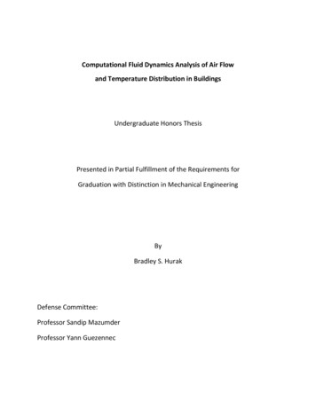
2MethodsA simple two-dimensional model of a room was analyzed using CFD-ACE TM, a commercialcomputational fluid dynamics software package, to examine airflow and temperature distribution underdifferent circumstances. The model was set in summer conditions in which cooling was necessary and inwinter conditions in which heating was necessary. In both cases, the position of the inlet and outletvents was parametrically changed yielding a large matrix of results.Additionally, a three-dimensional model was developed in much the same way as the twodimensional model. With the same number of inlet and outlet locations as the two-dimensional case, aparametric study was planned; however, computing time and convergence problems prevented thisstudy from being completed.2.1 Two-dimensional Model DescriptionA two-dimensional model of a rectangular room with a width of 12 feet and a height of 10 feet wasused to create a mesh with a density of approximately 7.5 nodes per linear foot. The resulting mesh was74 nodes wide by 92nodes high with a total of 6808 nodes. Additionally, the boundaries of the meshwere split into parts yielding ten one-foot-long sections that were used as inputs and outputs. Of thesesections, the inputs were located as follows: one inlet was located on the ceiling at 0.5 feet from the leftwall, one inlet was located on the floor at 0.5 feet from the left wall, and three inlets were located onthe left wall at 0.5 feet from the floor and ceiling and midway up the wall centered at 5 feet. The outletswere similarly located on the right side of the two-dimensional model. Also, a temperature monitorpoint that was used to determine the transient temperature at a location that would correspond to aperson sitting in a chair in the middle of the room was set at 3 feet above the floor and 6 feet fromeither side wall. Figure 1 shows the geometry of the two-dimensional model, including the locations ofthe inlets, which are denoted by the notation “I#”, where “I” stands for “inlet” and “#” is the number3
given to the inlet location, the outlets, which are similarly marked with the notation “O#”, and theplacement of the temperature probe, which is indicated with a “ ”.Figure 1: Two-dimensional model with inlets, outlets, and temperature probe.2.2 Three-dimensional Model DescriptionA three-dimensional model of a room in the shape of a rectangular prism was developed. Thephysical dimensions were set to be 12 feet wide by 12 feet long by 10 feet tall. The resulting mesh hadapproximately 5 nodes per linear foot, yielding a three-dimensional mesh of 152,460 nodes, or 82,080cells. This model also had inlet and outlet configurations that were analogous to the two-dimensionalcase. The inlets were located in one corner of the room while the outlets were in the opposite corner.The highest vent, for both inlets and outlets, was located in the corner of the ceiling of the model room4
at 6 inches from either sidewall. Moving down the wall, a vent was located at 6 inches below the ceilingand 6 inches from the sidewall while another vent was 6 inches above the floor and 6 inches from thesidewall. Also, there was a vent that was positioned in the middle of the height of the wall, centered at5 feet from the floor and with one edge 6 inches from the sidewall. Finally, another vent was located onthe floor at 6 inches from either sidewall. The inlets were sized at 1 foot by 1 foot while the outletswere 2 feet by 1 foot. A diagram of the three-dimensional model is shown in Figure 2. The inlets andoutlets are similarly identified as in the two-dimensional case presented above.Figure 2: Three-dimensional model with inlets and outlets.2.3 Parametric StudyUsing CFD-ACE , twenty five geometrically different cases were studied to evaluate the fluid flowand temperature distributions within the two-dimensional model room. These cases were5
parametrically determined from the above model; using only one inlet and one outlet for eachsimulation, the inlets and outlets were changed one at a time so that each case evaluated the model fora distinct combination of inlets and outlets.Table 1below identifies the twenty five test configurations that were considered.Table 1: List of test numbers according to inlet and outlet position.Inlet Outlet -43-54-14-24-34-44-55-15-25-35-45-52.4 Model ConditionsEach of the cases presented in Table 1 was simulated under hot and cold ambient temperatureconditions. In both cases, the target comfort condition was taken to be 295.2 K, or 72 F, based onindustry standards. For the two-dimensional case, transient simulations were carried out at stepintervals of 5 seconds for 360 time steps which is equivalent to 30 minutes. For the three-dimensionalmodel, steady state solutions were planned to be studied with transient analyses to follow. Adescription of the conditions and assumptions is given in the following sections.2.4.1Hot ConditionsThe hot conditions were meant to simulate a hot summer day. As such, a temperature of 308 K,or about 95 F, was chosen as the outside air temperature. Additionally, the ground temperature wasassumed to be cooler at 290 K, or approximately 62 F. The initial temperature inside the room wastaken to be equal to the external ambient condition at 308 K. The inlet temperature of the model ventswas set to be 2.3 K above the comfort condition at 298.5 K, or 77.6 F.6
2.4.2Cold ConditionsThe cold conditions were chosen to replicate cold winter temperatures. Thus, the ambienttemperature was set to 266.5 K, or 20 F. Also, the ground temperature was set slightly lower than thesummer ground condition at 286, or 55 F. Because heating is not completely turned off in coldconditions, the initial air temperature inside the room was taken to be 286 K. The inlet temperature wasset to be 2.2 K below the comfort condition at 292 K, or about 66 F.7
3CFD ModelThe CFD package, CFD-ACE , was set up to use three modules to resolve the flow and temperaturedistributions of the model: flow, heat transfer, and turbulence. Each of these three modules has its ownset of governing equations and is discussed in its respective section below. While the equationspresented apply directly to the two-dimensional cases, the three-dimensional cases require anequivalent set of three-dimensional equations.3.1 Flow ModuleThe flow module determines the velocity and pressure fields by solving the two-dimensionalmomentum equations and the pressure correction equations, respectively. These equations are guidedby the laws of conservation of mass and momentum, which lead to the use of the Navier-Stokesequations to iteratively resolve the flow solutions. The following sections describe the governing flowequations.3.1.1Mass Conservation EquationThe law of conservation of mass is applied to the model room which serves as the controlvolume; accordingly, the time rate of change of mass in the room must be balanced by the differencebetween the mass exiting and entering the room. This principle is described by the equation below.(1)where ρ is the air density andis the velocity vector. The first term on the left expresses the time rateof change of density while the second term describes the net mass flow through the control volume.3.1.2Momentum Conservation Equations8
The law of conservation of momentum must also be applied; this states that the time rate ofchange of momentum of a fluid element is equal to the sum of the forces acting on the element. Theequation below describes the two-dimensional x-component of this principle.(2)where u is the fluid velocity in the x-direction, p is the pressure, τ is the viscous stress, and S is the rateof increase in momentum caused by forces on the element. The left side of the equation is the rate ofchange of momentum in the x -direction while the left side describes the rate of change of total forceson the element in the x-direction. Similarly, the y-component is expressed below.(3)where v is the fluid velocity in the y-direction.3.1.3Navier-Stokes EquationsTo further develop the momentum equations given above, the variable viscous stresses for two-dimensional flows are defined below.(4)(5)(6)Combining equations 9 through 11 with momentum equations 7 and 8 results in the Navier-Stokesequations which are presented below.(7)9
(8)These above equations can be simplified and rewritten as the following equations.(9)(10)3.1.4Other Flow PropertiesThe following table shows the fluid properties that were held constant and used to calculateother model parameters.Table 2: Flow Model Constants.ParameterReference PressureUniversal Gas ConstantMolecular Weight of AirDynamic ViscositySpecific HeatThermal Conductivity of AirSymbolprefRMWμCpkairValue101325 Pa8.314472 J/mol K29 kg/kmol1.846(10-5) kg/m s1007 J/kg K0.0263 W/m KUsing the above values, other variable model parameters were calculated within the CFDsimulation. These calculations include the fluid density and the kinematic viscosity. The fluid densitywas calculated using the Ideal Gas Law. This equation is given below.(11)where ρ is density, p is pressure and T is the temperature of the air. Also, the kinematic viscosity wascalculated with the following equation.10
(12)3.2 Heat Transfer ModuleThe heat transfer module was used to calculate the temperature distribution within the modelroom as well as the interactions with the environment. These calculations were performed according tothe law of conservation of energy. The equation that was solved in CFD-ACE was the total enthalpyequation, which is given below.(13)where ho is the total enthalpy which is defined as:(14)where i is the internal energy, keff is the effective thermal conductivity, p is the static pressure, and τ isthe viscous stress tensor which was described in equations 9 through 11, above.3.2.1Thermal BoundariesIn addition to the above equations, it was necessary to define the conditions at the walls of theroom to determine the thermal interaction with the ambient temperature outside of the model. Theboundary consisted of three different elements: the ceiling, the walls, and the floor. While each ofthese sections had distinct thermal properties, a similar method of determining the effective heattransfer coefficients of each part was used. In general, an overall heat transfer coefficients wascalculated using a thermal resistance model which took into account the conductive heat transfer withineach layer of the boundary walls and the convective heat transfer to the ambient environment, ifapplicable. Overall, the heat transfer rate through the room’s boundaries can be expressed as follows:11
(15)where q is the heat transfer rate, heff is the overall heat transfer coefficient, A is the area of theboundary, Tw is the temperature on the inside of the boundary, and Tinf is the ambient temperature.Subsequently, the over heat transfer coefficient, heff, is defined as the reciprocal of the sum of thethermal resistances at the boundary, as shown in the equation below.(16)where the Rtotal is the combined conductive and convective thermal resistances, Rc and Rh, respectively.These properties are defined in the following equations.(17)where k is the material specific thermal conductivity and L is the thickness of the material layer.(18)where hinf is the convective heat transfer coefficient of air.Detailed below are the assumptions, values, and calculations used for each of these threesections.3.2.1.1 Ceiling Thermal PropertiesThe ceiling was simply modeled as three different layers of material and an external convectiveheat transfer layer as is shown in Figure 3, below. The type, thermal properties, and thickness of each ofthe materials is shown in the table below.12
Figure 3: Thermal resistance model of ceiling.Table 3: Material type, thermal properties and thickness of ceiling thermal model layers.Layer1234MaterialDrywallAirPlywoodAir (ambient)Thermal Propertiesk 0.1700 W/mKk 0.0263 W/mKk 0.1200 W/mKhinf 10 W/m2KThickness15.875 mm304.8 mm15.875 mmNAUsing this thermal resistance model and equations 3 and 4, the total thermal resistance of theceiling was calculated as follows:(19)Inserting the respective values yields a total thermal resistance of 11.915 m2K/W. The reciprocal of thisthermal resistance, as has been shown in equation 2, is the overall heat transfer coefficient of theceiling, hceiling, or 0.0839 W/m2K.3.2.1.2 Wall Thermal PropertiesThe thermal model of the walls consisted of four layers of material and an outer convective heattransfer layer. This concept is shown in Figure 4 and the layer properties are shown in Table 4 below.13
3Figure 4: Thermal resistance model of side walls.Table 4: Material type, thermal properties and thickness of side wall thermal model r (ambient)Thermal Propertiesk 0.1700 W/mKk 0.0263 W/mKk 0.1200 W/mKk 0.0940 W/mKh 10 W/m2KThickness15.875 mm101.60 mm15.875 mm15.875 mmNAUsing the above information and equations 2 through 4 as applied in the previous section, theoverall heat transfer coefficient of the side walls, hwall, was determined to be 0.3699 W/m2K.3.2.1.3 Floor Thermal PropertiesAgain, a similar thermal resistance model is used for the floor with the exception of theconvective heat transfer term which is not included in the formulation. Figure 5 shows that the floorwas taken to have five layers of material to a depth of approximately 6.5 feet, a depth at which theground temperature is considered to be constant. Table 5 shows the thermal and dimensionalproperties of the material layers.Figure 5: Thermal resistance model of floor.14
Table 5: Material type, thermal properties and thickness of floor thermal model eClayThermal Propertiesk 0.120 W/mKk 0.0263 W/mKk 1.0 W/mKk 1.4 W/mKk 1.3 W/mKThickness25.4 mm152.4 mm152.4 mm152.4 mm1.524 mUsing the information above, along with Equations 2 through 4, the overall heat transfercoefficient for the floor of the room, hfloor, was determined to be 0.1332 W/m2K.3.3 Turbulence ModuleThe CFD program was set to use a standard k-epsilon model for turbulence. The required inputvariables were the turbulent kinetic energy, K, and the turbulent dissipation, d. The equations used tofind these values are presented(20)where U is the flow velocity at the inlet and I is the turbulence intensity. The inlet flow velocity wastaken to be 1.5 air changes per hour, or ACH, meaning that the total volume of the room would bereplaced 1.5 times in one hour. The formulation for the inlet flow velocity, U, is shown below.(21)where is the required volumetric flow rate as calculated from equation 4 below and w is the width ofthe inlet.(22)where W is the room width and H is the room height. Inserting the respective values yields a volumetricflow rate, , equal to 16.7225 m2/hr, or 0.0046 m2/s. Plugging this value into equation 3 yields an inlet15
velocity, U, of 0.01524 m/s. This inlet flow velocity can be directly inserted into equation 6, with aturbulence intensity value of 0.05, to result in a turbulent kinetic energy value, K, of 8.71(10-7) m2/s2.Next, the turbulent dissipation, d, can be calculated using the equation 5.(23)where Cμ is a turbulence model constant of 0.09 and l is the turbulent length scale which is definedbelow.(24)where L is the characteristic length of the inlet. Using these relationships and the values above, theturbulent dissipation was calculated to be 1.4606(10-8) m2/s3.3.4 Three-dimensional Model PropertiesUsing the same formulations as presented above, the three-dimensional model properties thatwere different from the two-dimensional case are given in Table 6.Table 6: Three-dimensional model parameters.Parameter
Accordingly, this preliminary CFD model validation attempt was dismissed. The study by Sun et al. also provides a model of a CFD study of an indoor environment. A dynamic simulation was used to evaluate HVAC control systems based on a CFD model of a room, a mathematically modeled PID controller, and an actuation model.