Transcription
Efficient Belief Propagation for Utility Maximization and Repeated InferenceAniruddh Nath and Pedro DomingosDepartment of Computer Science and EngineeringUniversity of WashingtonSeattle, WA 98195-2350, U.S.A.{nath, pedrod}@cs.washington.eduAbstractMany problems require repeated inference on probabilistic graphical models, with different values for evidence variables or other changes. Examples of suchproblems include utility maximization, MAP inference,online and interactive inference, parameter and structure learning, and dynamic inference. Since smallchanges to the evidence typically only affect a small region of the network, repeatedly performing inferencefrom scratch can be massively redundant. In this paper, we propose expanding frontier belief propagation(EFBP), an efficient approximate algorithm for probabilistic inference with incremental changes to the evidence (or model). EFBP is an extension of loopybelief propagation (BP) where each run of inferencereuses results from the previous ones, instead of starting from scratch with the new evidence; messages areonly propagated in regions of the network affected bythe changes. We provide theoretical guarantees bounding the difference in beliefs generated by EFBP andstandard BP, and apply EFBP to the problem of expected utility maximization in influence diagrams. Experiments on viral marketing and combinatorial auctionproblems show that EFBP can converge much fasterthan BP without significantly affecting the quality of thesolutions.IntroductionMost work on approximate probabilistic inference in graphical models focuses on computing the marginal probabilities of a set of variables, or determining their most probablestate, given some fixed evidence and a fixed model. However, many interesting problems require repeated inference,with changing evidence or a changing model: Utility maximization (Howard and Matheson 2005) indecision networks involves a search over possible choicesof actions. We can treat each choice of actions as an assignment of truth values to evidence variables, and compute the expected utility of that choice by inferring theexpected values of the utility variables. Maximum a posteriori (MAP) inference (Park 2002),i.e., computing the most likely state of a set of query variables Q given partial evidence e of the variables in theCopyright c 2010, Association for the Advancement of ArtificialIntelligence (www.aaai.org). All rights reserved.complement of Q. We can treat the variables in Q aschanging evidence, and compute the likelihood for eachassignment of values to Q. Online inference, where the values of evidence variablesare repeatedly updated (possibly in real time). Interactive inference, where the choice of evidence variables, their values, and the choice of query can changearbitrarily as dictated by the user. Parameter and structure learning (Heckerman, Geiger,and Chickering 1995; Della Pietra, Della Pietra, and Lafferty 1997) involve repeatedly modifying the model andrecomputing the likelihood. Dynamic inference (Murphy 2002) involves sequentialproblems, where the query at one time step depends onevidence and hidden variables at that step and previousones.The obvious way to solve these problems is simply to repeatedly perform inference from scratch each time the evidence (or model) changes. However, if the problem remainslargely unchanged between two successive search iterations,it may be the case that most of the beliefs are not significantly altered by the changes. In these situations, it wouldbe beneficial to reuse as much of the computation as possiblebetween successive runs of inference.Delcher et al. (1996) presented an exact online inferencealgorithm for tree-structured Bayesian networks. Acar et al.(2008) refer to the problem of repeated inference on variations of a model as adaptive inference. They described anexact algorithm that updates marginals as the dependenciesin the model are updated. However, we are not aware ofany general-purpose approximate inference algorithms thatavoid redundant computation as the evidence changes. Inthis paper, we propose expanding frontier belief propagation (EFBP), an approximate inference algorithm that onlyupdates the beliefs of variables significantly affected by thechanged evidence. EFBP can be straightforwardly extendedto handle changes to the model. We provide guarantees onthe performance of EFBP relative to BP. These are based onthe fact that, if the potentials in a model are bounded, thedifference in marginal probabilities calculated by EFBP andtraditional loopy BP can be bounded as well.We apply EFBP to the problem of expected utility maximization in influence diagrams. Utility maximization can be
cast as repeated calculation of the marginals in a graphicalmodel with changing evidence. Under certain conditions, itcan be shown that the same actions are chosen whether BP orEFBP is used to calculate the marginals. Experiments in viral marketing and combinatorial auction domains show thatEFBP can be orders of magnitude faster than BP, withoutsignificantly affecting the quality of the solutions.Graphical Models and Decision TheoryGraphical models compactly represent the joint distributionof a set of variables X (X1 , X2 , . . . , Xn ) XQas a product of factors (Pearl 1988): P (X x) Z1 k φk (xk ),where each factor φk is a non-negative function of a subset of the variables xk , and Z is a normalization constant.Under appropriate restrictions, the model is a Bayesian network and Z 1. A Markov network or Markov random field can have arbitrary factors. Graphical modelscan alsoPbe represented in log-linear form: P (X x) 1i wi gi (x)), where the features gi (x) are arbitraryZ exp (functions of the state.A key inference task in graphical models is computingthe marginal probabilities of some variables (the query)given the values of some others (the evidence). This problem is #P-complete, but can be solved approximately usingloopy belief propagation (BP) (Yedidia, Freeman, and Weiss2003). In the simplest form, the Markov network is first converted to an equivalent pairwise network. Belief propagationthen works by repeatedly passing messages between nodesin this network. The message from node t to node s is:XYmts (xs ) φts (xt , xs )φt (xt )mut (xt )xtu nb(t)\{s}where nb(t) is the set of neighbors of t. The (unnormalized)belief at node t is given by: Mt (xt ) Qφt (xt ) u nb(t) mut (xt ).Many message-passing schedules are possible; the mostwidely used one is flooding, where all nodes send messagesat each step. In general, belief propagation is not guaranteedto converge, and it may converge to an incorrect result, butin practice it often approximates the true probabilities well.An influence diagram or decision network is a graphicalrepresentation of a decision problem (Howard and Matheson 2005). It consists of a Bayesian network augmentedwith two types of nodes: decision or action nodes and utilitynodes. The action nodes represent the agent’s choices; factors involving these nodes and state nodes in the Bayesiannetwork represent the (probabilistic) effect of the actions onthe world. Utility nodes represent the agent’s utility function, and are connected to the state nodes that directly influence utility.The fundamental inference problem in decision networks is finding the assignment of values to the action nodes that maximizes the agent’s expected utility, possibly conditioned on some evidence. If a is achoice of actions, e is the evidence, x is a state, andU (x a, e) is the utility of x given a and e, then theMEU problemis to compute argmaxa E[U (x a, e)] Pargmaxa x P (x a, e)U (x a, e).Expanding Frontier Belief PropagationThe repeated inference problem deals with inference withchanging evidence, changing model parameters or changinggraph structure. For simplicity, we will focus on the casewhere the evidence changes and the choice of evidence variables is fixed, as are the parameters and structure; our formulation can be straightforwardly extended to incorporatethese other kinds of variation.Let G be a graphical model on the variables in X.E X is the evidence set. We are given a sequence e (e1 , . . . , e e ), each element of which is an assignmentof values to the variables in E. For each element ek of e,we wish to infer the marginal probabilities of the variablesin X\E, given that E ek .Changing the values of a small number of evidence nodesis unlikely to significantly change the probabilities of moststate nodes in a large network. EFBP takes advantage ofthis by only updating regions of the network affected bythe new evidence. The algorithm starts by computing themarginal probabilities of non-evidence nodes given the initial evidence values using standard BP (e.g., by flooding).Then, each time the evidence is changed, it maintains a set of nodes affected by the changed evidence variables, initialized to contain only those changed nodes. In each iteration of BP, only the nodes in send messages. Neighbors ofnodes in are added to if the messages they receive differby more than a threshold γ from the final messages they received when they last participated in BP. (The neighbors ofa node are the nodes that appear in some factor with it, i.e.,its Markov blanket.) In the worst case, the whole networkmay be added to , and we revert to BP. In most domains,however, the effect of a change usually dies down quickly,and only influences a small region of the network. In suchsituations, EFBP can converge much faster than BP.Pseudocode for EFBP is shown in Algorithm 1. m̂k,its isthe message from node t to node s in iteration i of inferkence run k. m̂k,cis the final message sent from t to s intsinference run k. (If s was not in in inference run k, thenk 1,ckm̂k,c m̂ts k 1 .) To handle changes to the model fromtsone iteration to the next, we simply add to variables directly affected by that change (e.g., the child variable of anew edge when learning a Bayesian network).EFBP is based on a similar principle to residual beliefpropagation (RBP) (Elidan, McGraw, and Koller 2006): focus effort on the regions of the graph that are furthest fromconvergence. However, while RBP is used to schedule message updates in a single run of belief propagation, the purpose of EFBP is to minimize redundant computation whenrepeatedly running BP on the same network, with varyingsettings of some of the variables. One could run EFBP using RBP to schedule messages, to speed up convergence.If the potentials are bounded, EFBP’s marginal probability estimates provide bounds on BP’s. We can show thisby viewing the difference between the beliefs generated byEFBP and those generated by BP as multiplicative error inthe messages passed by EFBP:k,iim̂k,its (xs ) m̃ts (xs )ẽts (xs )
Algorithm 1 EFBP(variables X, graphical model G, evidence e, threshold γ)m̂1,1tsfor all t, s: 1Perform standard BP on X and G with evidence e1 .for k 2 to e dok 1,ck 1for all t, s: m̂k,1ts m̂ts set of evidence nodes that changebetween ek and ek 1converged Falsei 1while converged False doSend messages from all nodes in ,given evidence ekconverged Truefor all nodes s that receive messages dok 1,ck 1if m̂k,i γ for any t nb(s) thents m̂tsInsert s into end ifk,i 1if s and m̂k,i γts m̂tsfor any t nb(s) thenconverged Falseend ifend fori i 1end whileend forwhere m̂k,its (xs ) is the message sent by EFBP in iteration iof inference run k (i.e., nodes not in effectively resend thesame messages as in i 1); m̃k,its (xs ) is the message sent ifall nodes recalculate their messages in iteration i, as in BP;and ẽits (xs ) is the multiplicative error introduced in iterationi of EFBP.This allows us to bound the difference in marginal probabilities calculated by BP and EFBP. For simplicitly, weprove this for the special case of binary nodes. The proofuses a measure called the dynamic range of a function, defined as follows (Ihler, Fisher, and Willsky 2005):pd(f ) sup f (x)/f (y)x,yTheorem 1. For binary node xt , the probability estimatedby BP at convergence (pt ) can be bounded as follows interms of the probability estimated by EFBP (p̂t ) after n iterations:1pt lb(pt )n2(ζt ) [(1/p̂t ) 1] 11pt ub(pt )(1/ζtn )2 [(1/p̂t ) 1] 1Pn1where log ζtn u nb(t) log νut, νts δ(ẽ1ts )d(φts )2 , andiνut is given by:d(φts )2 εits 1i 1log νts log log δ(ẽits )d(φts )2 εitsXilog εits log νutu nb(t)\sδ(ẽits )v uu 1 γ/ m̃k,i(x)stsu sup txs ,ys1 γ/ m̃k,its (ys )Proof.k,iSince EFBP recalculates messages when m̂k,its m̃ts γ,m̃k,its (xs ) γ k,iim̃k,its (xs )ẽts (xs ) m̃ts (xs ) γ1 γ/m̃k,its (xs ) 1 γ/m̃k,its (xs )ẽits (xs )This allows us to bound the dynamic range of ẽits :v uu 1 γ/ m̃k,i(x)stsu δ(ẽits )d(ẽits ) sup tk,ixs ,ys1 γ/ m̃ts (ys )Theorem 15 of Ihler et al. (2005) implies that, for any fixedpoint beliefs {Mt } found by belief propagation, after n 1iterations of EFBP resulting in beliefs {M̂tn } we haveXnlog νut log ζtnlog d(Mt /M̂tn ) u nb(t)It follows that d(Mt /M̂tn )Mt (1)/M̂tn (1)Mt (0)/M̂tn (0) ζtn , and therefore (ζtn )2 and (1 p̂t )/p̂t (ζtn )2 (1 pt )/pt ,where pt and p̂t are obtained by normalizing Mt and M̂t .The upper bound follows, and the lower bound can be obtained similarly.ican be thought of as a measure of the acIntuitively, νutcumulated error in the incoming message from u to t in iteration i. It can be computed iteratively using a messagepassing algorithm similar to BP.Maximizing Expected UtilityThe MEU problem in influence diagrams can be cast as a series of marginal probability computations with changing evidence. If ui (xi ) and pi (xi a, e) are respectively the utilityand marginal probability of utility node i’s parents Xi taking values xi , then the expected utility of an action choiceis:XE[U (a e)] P (x a, e)U (x a, e)x XP (x a, e)XXx XXi ixiXXiui (xi )X1{Xi xi }ui (xi )xi1{Xi xi }P (x a, e)xui (xi )pi (xi a, e)xiGiven a choice of actions, we can treat action nodes as evidence. To calculate the expected utility, we simply need tocalculate the marginal probabilities of all values of all utilitynodes. Different action choices can be thought of as different evidence.In principle, the MEU action choice can be found bysearching exhaustively over all action choices, computing
the expected utility of each using any inference method.However, this will be infeasible in all but the smallest domains. An obvious alternative, particularly in very largedomains, is greedy search: starting from a random actionchoice, consider flipping each action in turn, do so if it increases expected utility, and stop when a complete cycle produces no improvements. This is guaranteed to converge to alocal optimum of the expected utility, and is the method weuse in our experiments.Lemma 2. The expected utility Ebp [U ] of an action choiceestimated by BP can be bounded as follows:hXXEbp [U ] ui (xi ) 1{ui (xi ) 0}lb(pi (xi a, e))ixii 1{ui (xi ) 0}ub(pi (xi a, e))hXXEbp [U ] ui (xi ) 1{ui (xi ) 0}ub(pi (xi a, e))ixi 1{ui (xi ) 0}lb(pi (xi a, e))iBased on this lemma, we can design a variant of EFBPthat is guaranteed to produce the same action choice as BPwhen used with greedy search. Let Ai denote the set ofaction choices considered in the ith step of greedy search. IfEFBP picks action choice a Ai , BP is guaranteed to makethe same choice if the following condition holds:a AiExperimentsWe evaluated the performance of EFBP on two domains: viral marketing and combinatorial auctions. We implementedEFBP as an extension of the Alchemy system (Kok et al.2008). The experiments were run on 2.33 GHz processorswith 2 GB of RAM. We used a convergence threshold of10 4 for flooding, including the initial BP run for EFBP,and a threshold of γ 10 3 for the remaining iterationsof EFBP. We evaluated the utility of the actions chosen byEFBP using a second run of full BP, with a threshold of10 4 . As is usually done, both algorithms were run for afew (10) iterations after the convergence criterion was met.Viral MarketingProof. The lemma follows immediately from Theorem 1and the definition of expected utility.lb(E[U (a)]) maxub(E[U (a0 )])0In practice, EFBP is unlikely to provide large speedupsover BP, since the bound in Theorem 1 must be repeatedlyrecalculated even for nodes outside . Empirically, runningEFBP with a fixed threshold not much higher than BP’s convergence threshold seems to yield an action choice of verysimilar utility to BP’s in a fraction of the time.(1)When the condition does not hold, we revert the messagesof all nodes to their values after the initial BP run, insert allchanged actions into , and rerun EFBP. If condition 1 stilldoes not hold, we halve γ and repeat. (If γ becomes smallerthan the BP convergence threshold, we run standard BP.) Wecall this algorithm EFBP .Note that using the above bound for search requires a1slight modification to the calculation of νts, since EFBPand BP result in different message initializations for thefirst BP iteration at every search step. If BP initializes allmessages to 1 before every search step, the error functionẽ1ts (xs ) m̂k,1ts (xs ). If BP initializes its messages withtheir values from end of the previous search iteration, then1iνtscan also be similarly initialized. The calculations of νtsfor i 6 1 are not altered.Let Greedy(I) denote greedy search using inferencealgorithm I to compute expected utilities.Theorem 3. Greedy(EFBP ) outputs the same actionchoice as Greedy(BP).Proof. Condition 1 guarantees that EFBP makes the sameaction choice as BP. Since EFBP guarantees that the condition holds in every iteration of the final run of EFBP, itguarantees that the action choice produced is the same.Viral marketing is based on the premise that members of asocial network influence each other’s purchasing decisions.The goal is then to select the best set of people to marketto, such that the overall profit is maximized by propagationof influence through the network. Originally formalized byDomingos and Richardson (2001), this problem has sincereceived much attention, including both empirical and theoretical results.A standard dataset in this area is the Epinions web oftrust (Richardson and Domingos 2002). Epinions.com is aknowledge-sharing Web site that allows users to post andread reviews of products. The “web of trust” is formed byallowing users to maintain a list of peers whose opinionsthey trust. We used this network, containing 75,888 usersand over 500,000 directed edges, in our experiments. Withover 75,000 action nodes, this is a very large decision problem, and no general-purpose MEU algorithms have previously been applied to it (only domain-specific implementations).We used a model very similar to that of Domingos andRichardson (2001). We represent this problem as a loglinear model with one binary state variable bi representingthe purchasing decision of each user i (i.e., whether or notthey buy the product). The model also has one binary actionvariable mi for each user, representing the choice of whetheror not to market to that person. The prior belief about eachuser’s purchasing decision is represented by introducing asingleton feature for that user. The value is 1 if the user buysthe product, and 0 otherwise. In our experiments, this feature had a weight of 2. The effect of the marketing actionson the users’ purchasing decisions is captured by a secondset of features. For each user, we introduce a feature whosevalue is 1 when the formula mi bi is true, and 0 otherwise (i.e., when the user is marketed to but does not buy theproduct). All these features are given the same weight, w1 .The web of trust is encoded as a set of pairwise featuresover the state variables. For each pair of users (i, j) such that
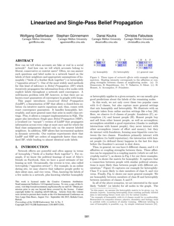
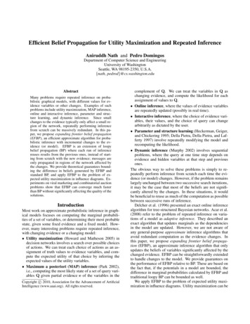
10000BTime (hrs)MUMUB10001001010.6EFBPBP0.70.80.9Influence weight1(a)Figure 1: Influence diagram for viral marketing.i trusts j, the value of the feature is 1 when the formula bj bi is true, and 0 otherwise (i.e., j buys the product but i doesnot.) These features represent the fact that if j purchases theproduct, i is more likely to do so as well. These features allhave weight w2 .For each user, we also introduce two utility nodes. Thefirst represents the cost of marketing to the user, and thesecond represents the profit from each purchase. The firstutility node is connected to the action node correspondingto the user, and the second is connected to the state noderepresenting the user’s purchasing decision. We set the costof marketing to each user to 1, and the profit from eachpurchase to 20.Note that since this model is not locally normalized, it isnot a traditional influence diagram. However, it is equivalentto an influence diagram with four nodes (see Figure 1): An action node M whose state space is the set of possiblemarketing choices over all users. A corresponding utility node UM , representing the costof each marketing choice. A state node B, representing the set of possible purchasing decisions by the users. A corresponding utility node UB , representing the profitfrom each possible purchasing decision.The log-linear model described above can be thought of asa compact representation of the conditional probability distributions and utility functions for this four-node influencediagram.We ran greedy search with BP and EFBP directly on thismodel. The initial action choice was to market to no one.All results are averages of five runs. Fixing w1 at 0.8 forall users, inference times varied as shown in Figure 2(a) aswe changed w2 . Running utility maximization with BP untilconvergence was not feasible; instead, we extrapolated fromthe number of actions considered during the first 24 hours,assuming that search with BP would consider the same number of actions as search with EFBP. Figure 2(b) plots the result of a similar experiment, with w2 fixed at 0.6 and varyingw1 . In both cases, EFBP was consistently orders of magnitude faster than BP.We can also compare the utility obtained by BP and EFBPgiven a fixed running time of 24 hours. EFBP consistentlyachieves about 40% higher utility than BP when varying theinfluence weight, with higher advantage for lower weights.Time (hrs)1000010001001010.6EFBPBP0.70.80.9Marketing weight1(b)Figure 2: Convergence times for viral marketing.For a marketing weight of 1.0, EFBP achieves about 80%higher utility than BP; this advantage decreases gradually tozero as the weight is reduced (reflecting the fact that fewerand fewer customers buy).Richardson and Domingos (2002) tested various speciallydesigned algorithms on the same network. They estimatedthat inference using the model and algorithm of Domingosand Richardson (2001), which are the most directly comparable to ours, would have taken hundreds of hours to converge (100 per pass). (This was reduced to 10-15 minutes using additional problem-specific approximations, and a muchsimpler linear model that did not require search was evenfaster.) Although these convergence times cannot be directlycompared with our own (due to the different hardware, parameters, etc., used), it is noteworthy that EFBP convergesmuch faster than the most general of their methods.Probabilistic Combinatorial AuctionsCombinatorial auctions can be used to solve a wide variety of resource allocation problems (Cramton, Shoham, andSteinberg 2006). An auction consists of a set of bids, eachof which is a set of requested products and an offered reward. The seller determines which bids to assign each product to. When all requested products are assigned to a bid,the bid is said to be satisfied, and the seller collects the reward. The seller’s goal is to choose an assignment of products to bids that maximizes the sum of the rewards of satisfied bids; this is an NP-hard problem. While there hasbeen much research on combinatorial auctions, it generallyassumes that the world is deterministic (with a few exceptions, e.g., Golovin (2007)). In practice, however, both thesupply and demand for products are subject to many sources
24ity maximization (e.g., online inference, learning, etc.), andapplying it to other domains.Time (mins)2016AcknowledgementsEFBPBP12840012 3 4 5 6Competition weight78Figure 3: Convergence times for combinatorial auctions.of uncertainty. (For example, supply of one product maymake supply of another less likely because they compete forresources.)We model uncertainty in combinatorial auctions by allowing product assignments to fail, resulting in the loss ofreward from the corresponding bids. The model containsone multi-valued action for each product, with one possible value for each bid. Each product also has a binary statevariable, to model the success or failure of the action corresponding to that product.To model competition between pairs of products, we introduce a set of pairwise features. The features have value 1when one or both of the product assignments fail. In otherwords, the success of one increases the failure probability ofthe other. These features create a network of dependenciesbetween product failures.The model also contains one binary utility node for eachbid. Note that, as in the viral marketing experiment, thismodel does not yield a traditional influence diagram. However, it can similarly be converted to an equivalent influencediagram with a small number of high-dimensional nodes.We generated bids according to the decay distribution described by Sandholm (2002), with α 0.75, and randomlygenerated 1000 competition features from a uniform distribution over product pairs. Figure 3 plots the inference timefor a 1000-product, 1000-bid auction, varying the weightof the competition features. The results are averages of tenruns. As in the viral marketing experiment, EFBP convergesmuch faster than BP. Since in this case both algorithms canbe run until convergence, the expected utilities of the chosenproduct assignments are extremely similar.ConclusionIn this paper, we presented expanding frontier belief propagation, an efficient approximate algorithm for probabilistic inference with incremental changes to the evidence ormodel. EFBP only updates portions of the graph significantly affected by the changes, thus avoiding massive computational redundancy. We applied this algorithm to utilitymaximization problems, and provided theoretical bounds onthe quality of the solutions.Directions for future work include extending the “expanding frontier” idea to other kinds of inference algorithms(e.g., MCMC), applying it to other problems besides util-This research was partly funded by ARO grant W911NF08-1-0242, AFRL contract FA8750-09-C-0181, DARPA contracts FA8750-05-2-0283, FA8750-07-D-0185, HR0011-06-C0025, HR0011-07-C-0060 and NBCH-D030010, NSF grants IIS0534881 and IIS-0803481, and ONR grant N00014-08-1-0670.The views and conclusions contained in this document are thoseof the authors and should not be interpreted as necessarily representing the official policies, either expressed or implied, of ARO,DARPA, NSF, ONR, or the United States Government.ReferencesAcar, U. A.; Ihler, A. T.; Mettu, R. R.; and S̈umer, O. 2008. Adaptive inference on general graphical models. In Proc. of UAI-08.Cramton, P.; Shoham, Y.; and Steinberg, R. 2006. CombinatorialAuctions. MIT Press.Delcher, A. L.; Grove, A. J.; Kasif, S.; and Pearl, J. 1996.Logarithmic-time updates and queries in probabilistic networks.Journal of Artificial Intelligence Research 4:37–59.Della Pietra, S.; Della Pietra, V.; and Lafferty, J. 1997. Inducingfeatures of random fields. IEEE Transactions on Pattern Analysisand Machine Intelligence 19:380–392.Domingos, P., and Richardson, M. 2001. Mining the network valueof customers. In Proc. of KDD-01.Elidan, G.; McGraw, I.; and Koller, D. 2006. Residual belief propagation: Informed scheduling for asynchronous message passing.In Proc. of UAI-06.Golovin, D. 2007. Stochastic packing-market planning. In Proc.of EC-07.Heckerman, D.; Geiger, D.; and Chickering, D. M. 1995. LearningBayesian networks: The combination of knowledge and statisticaldata. Machine Learning 20:197–243.Howard, R. A., and Matheson, J. E. 2005. Influence diagrams.Decision Analysis 2(3):127–143.Ihler, A. T.; Fisher, J. W.; and Willsky, A. S. 2005. Loopy beliefpropagation: Convergence and effects of message errors. Journalof Machine Learning Research 6:905–936.Kok, S.; Sumner, M.; Richardson, M.; Singla, P.; Poon, H.; Lowd,D.; Wang, J.; and Domingos, P. 2008. The Alchemy system for statistical relational AI. Technical report, University of , K. P. 2002. Dynamic Bayesian Networks: Representation,Inference and Learning. Ph.D. Dissertation, University of California, Berkeley.Park, J. 2002. MAP Complexity Results and Approximation Methods. In Proc. of UAI-02.Pearl, J. 1988. Probabilistic Reasoning in Intelligent Systems:Networks of Plausible Inference. Morgan Kaufmann.Richardson, M., and Domingos, P. 2002. Mining knowledgesharing sites for viral marketing. In Proc. of KDD-02.Sandholm, T. 2002. Algorithm for optimal winner determinationin combinatorial auctions. Artificial Intelligence 135:1–54.Yedidia, J. S.; Freeman, W. T.; and Weiss, Y. 2003. Understandingbelief propagation and its generalizations. In Exploring ArtificialIntelligence in the New Millenium. Science and Technology Books.
the world. Utility nodes represent the agent's utility func-tion, and are connected to the state nodes that directly influ-ence utility. The fundamental inference problem in decision net-works is finding the assignment of values to the ac-tion nodes that maximizes the agent's expected util-ity, possibly conditioned on some evidence. If a is a