WIXLIB

underlying problem is then: How can we assign class labels when we know who-contacts-whom and the apriori (“explicit”) labels for some of the nodes in the network ? Thislearning scenario, where we reason from observed trainingcases directly to test cases, is also called transductive inference, or semi-supervised learning (SSL).3One of the most widely used methods for this kind oftransductive inference in networked data is Belief Propagation (BP) [44], which has been successfully applied in scenarios, such as fraud detection [32, 38] and malware detection [5]. BP propagates the information from a few explicitlylabeled nodes throughout the network by iteratively propagating information between neighboring nodes. However,BP has well-known convergence problems in graphs withloops (see [44] for a detailed discussion from a practitioner’spoint of view). While there is a lot of work on convergenceof BP (e.g., [8, 34]), exact criteria for convergence are notknown [35, Sec. 22]. In addition, whenever we get additionalexplicit labels (e.g., we identify more fraudsters in the onlineauction setting), we need to re-run BP from scratch. Theseissues raise fundamental theoretical questions of practicalimportance: How can we find sufficient and necessary conditions for convergence of the algorithm? And how can wesupport fast incremental updates for dynamic networks?Contributions. This paper introduces two new formulations of BP. Unlike standard BP, these (i) come with exact convergence guarantees, (ii) allow closed-form solutions,(iii) give a clear intuition about the algorithms, (iv) can beimplemented on top of standard SQL, and (v) one can evenbe updated incrementally. In more detail, we introduce:(1) LinBP : Section 3 gives a new matrix formulation formulti-class BP called Linearized Belief Propagation (LinBP).Section 4 proves LinBP to be the result of applying a certainlinearization process to the update equations of BP. Section 4.2 goes one step further and shows that the solutionto LinBP can be obtained in closed-form by the inversionof an appropriate Kronecker product. Section 5.1 showsthat this new closed-form provides us with exact convergence guarantees (even on graphs with loops) and a clear intuition about the reasons for convergence/non-convergence.Section 5.3 shows that our linearized matrix formulation ofLinBP allows a compact implementation in SQL with standard joins and aggregates, plus iteration. Finally, experiments in Sect. 7 show that a main-memory implementationof LinBP takes 4 sec for a graph for which standard BPtakes 40 min, while giving almost identical classifications( 99.9% overlap).(2) SBP : Section 6 gives a novel semantics for “local” (or“myopic”) transductive reasoning called Single-pass BeliefPropagation (SBP). SBP propagates information across every edge at most once (i.e. it ignores some edges) and is ageneralization of relational learners [31] from homophily toheterophily and even more general couplings between classesin a sound and intuitive way. In particular, the final labelsdepend only on the nearest neighbors with explicit labels.The intuition is simple: If we do not know the political leanings of Alice’s friends, than knowing the political leaning offriends of Alice’s friends (i.e. nodes that are 2 hops awayin the underlying network) will help us make some predictions about her. However, if we do know about most of herfriends, then information that is more distant in the networkcan often be safely ignored. We formally show the connection between LinBP and SBP by proving that the labelingassignments for both are identical in the case of decreasingaffinities between nodes in a graph. Importantly, SBP (incontrast to standard BP and LinBP) allows fast incrementalmaintenance for the predicated labels if the underlying network is dynamic: Our SQL implementation of SBP allowsincremental updates with an intuitive index based on shortest paths to explicitly labeled nodes. Finally, experimentsin Sect. 7 show that a disk-bound implementation of SBPis even faster than LinBP by one order of magnitude whilegiving similar classifications ( 98.6% overlap).Outline. Sect. 2 provides necessary background on BP.Sect. 3 introduces the LinBP matrix formulation. Sect. 4sketches its derivation. Sect. 5 provides convergence guarantees, extends LinBP to weighted graphs, and gives a SQLimplementation of LinBP. Sect. 6 introduces the SBP semantics, including a SQL implementation for incrementalmaintenance. Sect. 7 gives experiments. Sect. 8 contrastsrelated work, and Sect. 9 concludes. All proofs plus anadditional algorithm for incrementally updating SBP whenadding edges to the graph are available in our technical report on ArXiv [13]. The actual SQL implementations ofLinBP and SBP are available on the authors’ home pages.Belief Propagation (BP), also called the sum-product algorithm, is an exact inference method for graphical models with tree structure [40]. The idea behind BP is thatall nodes receive messages from their neighbors in parallel,then they update their belief states, and finally they sendnew messages back out to their neighbors. In other words,at iteration i of the algorithm, the posterior belief of a nodes is conditioned on the evidence that is i steps away from sin the underlying network. This process repeats until convergence and is well-understood on trees.When applied to loopy graphs, however, BP is not guaranteed to converge to the marginal probability distribution.Indeed, Judea Pearl, who invented BP, cautioned about theindiscriminate use of BP in loopy networks, but advocatedto use it as an approximation scheme [40]. More important,loopy BP is not even guaranteed to converge at all. Despitethis lack of exact criteria for convergence, many papers havesince shown that “loopy BP” gives very accurate results inpractice [49], and it is thus widely used today in variousapplications, such as error-correcting codes [29] or stereoimaging in computer vision [9]. Our practical interest in BPcomes from the fact that it is not just an efficient inferencealgorithm on probabilistic graphical models, but it has alsobeen successfully used for transductive inference.The transductive inference problem appears, in its generality, in a number of scenarios in both the database andmachine learning communities and can be defined as follows:Consider a set of keys X {x1 , . . . , xn }, a domain of valuesY {y1 , . . . , yk }, a partial labeling function : XL Ywith XL X that maps a subset of the keys to values,a weighted mapping w : (X1 , X2 ) R with (X1 , X2 ) X X, and a local condition fi (X, w, xi , i ) that needs tohold for a solution to be accepted.4 The three problems arethen to find: (i) an appropriate semantics that determines3Contrast this with inductive learning, where we first infer generalrules from training cases, and only then apply them to new test cases.4Notice that update equations define a local condition implicitly bygiving conditions that a solution needs to fulfill after convergence.2.582BELIEF PROPAGATION

Formulalabels for all keys, (ii) an efficient algorithm that implementsthis semantics, and (iii) efficient ways to update labels incase the labeling function , or the mapping w change.In our scenario, we are interested in the most likely beliefs(or classes) for all nodes in a network. BP helps to iterativelypropagate the information from a few nodes with explicitbeliefs throughout the network. More formally, consider agraph of n nodes (or keys) and k possible classes (or values).Each node maintains a k-dimensional belief vector whereeach element i represents a weight proportional to the beliefthat this node belongs to class i. We denote by es the vectorof prior (or explicit) beliefs and bs the vector of posterior(or implicit or final ) beliefs at nodethat esP s, and requirePand bs are normalized to 1; i.e. i es (i) i bs (i) 1.5Using mst for the k-dimensional message that node s sendsto node t, we can write the BP update formulas [35, 48]for the belief vector of each node and the messages it sendsw.r.t. class i as:Y1es (i)mus (i)(1)bs (i) Zsu N (s)XYmst (i) Hst (j, i) es (j)mus (j)(2)j2Division31 1k1 2Approx. ( k1 1 )(1 2 22 . . .) 1 1 k2kFigure 2: Two linearizing approximations used in our derivation.In this section, we introduce Linearized Belief Propagation(LinBP), which is a closed-form description for the final beliefs after convergence of BP under mild restrictions of ourparameters. The main idea is to center values around default values (using Maclaurin series expansions) and to thenrestrict our parameters to small deviations from these defaults. The resulting equations replace multiplication withaddition and can thus be put into a matrix framework witha closed-form solution. This allows us to later give exactconvergence criteria based on problem parameters.Definition 2 (Centering). We call a vector or matrix x“ centered around c” if all its entries are close to c and theiraverage is exactly c.Definition 3 (Residual vector/matrix). If a vector x is centered around c, then the residual vector around c is definedas x̂ [x1 c, x2 c, . . .]. Accordingly, we denote a matrix X̂ as a residual matrix if each column and row vectorcorresponds to a residual vector.u N (s)\tHere, we write Zs for a normalizer that makes the elements of bs sum up to 1, and Hst (j, i) for a proportional“coupling weight” that indicates the relative influence ofclass j of node s on class i of node t (cf. Fig. 1).6 We assume that the relative coupling between classes is the samein the whole graph; i.e. H(j, i) is identical for all edges inthe graph. We further require this coupling matrix H to bedoubly stochastic and symmetric: (i) Double stochasticity isa necessary requirement for our mathematical derivation.7(ii) Symmetry is not required but follows from our assumption of undirected edges. For BP, the above update formulasare then repeatedly computed for each node until the values(hopefully) converge to the final beliefs.The goal in our paper is to find the top beliefs for eachnode in the network, and to assign these beliefs to the respective nodes. That is, for each node s, we are interestedin determining the classes with the highest values in bs .For example, we call the vector x [1.01, 1.02, 0.97] centered around c 1.8 The residuals from c will form theresidual vector x̂ [0.01, 0.02, 0.03]. Notice that the entries in a residual vector always sum up to 0, by construction.The main ideas in our proofs are as follows: (1) the kdimensional message vectors m are centered around 1; (2)all the other k-dimensional vectors are probability vectors,they have to sum up to 1, and thus they are centered around1/k. This holds for the belief vectors b, e, and for the allentries of matrix H; and (3) we make use of each of the twolinearizing approximations shown in Fig. 2 exactly once.According to aspect (1) of the previous paragraph, werequire that the messages sent are normalized so that theaverage value of the elements of a message vector is 1 or,equivalently, that the elements sum up to k:Y1 XH(j, i) es (j)mus (j)(3)mst (i) Zst jProblem 1 (Top belief assignment). Given: (1) an undirected graph with n nodes and adjacency matrix A, whereA(s, t) 6 0 if the edge s t exists, (2) a symmetric, doublystochastic coupling matrix H representing k classes, whereH(j, i) indicates the relative influence of class j of a nodeon class i of its neighbor, and (3) a matrix of explicit beliefsE, where E(s, i) 6 0 is the strength of belief in class i bynode s. The goal of top belief assignment is to infer foreach node a set of classes with highest final belief.u N (s)\tHere, we write Zst as a normalizer that makes the elementsof mst sum up to k. Scaling all elements of a message vectorby the same constant does not affect the resulting beliefssince the normalizer in Eq. 1 makes sure that the beliefs arealways normalized to 1, independent of the scaling of themessages. Thus, scaling messages still preserves the exactsolution, yet it will be essential for our derivation.In other words, our problem is to find a mapping from nodesto sets of classes (in order to allow for ties).3.Maclaurin seriesLogarithm ln(1 ) 2 3 . . .Theorem 4 (Linearized BP (LinBP)). Let B̂ and Ê be theresidual matrices of final and explicit beliefs centered around1/k, Ĥ the residual coupling matrix centered around 1/k, Athe adjacency matrix, and D diag(d) the diagonal degreematrix. Then, the final belief assignment from belief propagation is approximated by the equation system:LINEARIZED BELIEF PROPAGATIONP5Notice thati as shortP here and in the rest of this paper, we writeform forwheneverkisclearfromthecontext.i [k]6We chose the symbol H for the coupling weights as reminder ofour motivating concepts of homophily and heterophily. Concretely,if H(i, i) H(j, i) for j 6 i, we say homophily is present, otherwiseheterophily or a mix between the two.7Notice that single-stochasticity could easily be constructed by takingany set of vectors of relative coupling strengths between neighboringclasses, normalizing them to 1, and arranging them in a matrix.2B̂ Ê AB̂Ĥ DB̂Ĥ(LinBP) (4)8All vectors x in this paper are assumed to be column vectors[x1 , x2 , . . .] even if written as row vectors [x1 , x2 , . . .].583

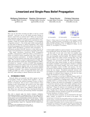
ktt nkstnsnB̂ Ê kk nktnknB̂ Ĥ k Ĥ(j, i), e(i) k1 ê(i), and b(i) k1 b̂(i).10 As aconsequence, Ĥ Rk k is the residual coupling matrix thatmakes explicit the relative attraction and repulsion: Thesign of Ĥ(j, i) tells us if the class j attracts or repels classi in a neighbor, and the magnitude of Ĥ(j, i) indicates thestrength. Subsequently, this centering allows us to rewritebelief propagation in terms of the residuals.1kk nAtnD2B̂ ĤFigure 3: LinBP equation (Eq. 4): Notice our matrix conventions:Ĥ(j, i) indicates the relative influence of class j of a node on classi of its neighbor, A(s, t) A(t, s) 6 0 if the edge s t exists, andB̂(s, i) is the belief in class i by node s.Lemma 5 (Centered BP). By centering the coupling matrix, beliefs and messages, the equations for belief propagation can be approximated by:1 Xm̂us (i)(8)b̂s (i) ês (i) ku N (s)XXm̂st (i) kĤ(j, i)b̂s (j) Ĥ(j, i)m̂ts (j)(9)Figure 3 illustrates Eq. 4 and shows our matrix conven2tions. We refer to the term DB̂Ĥ as “echo cancellation”.9For increasingly small residuals, the echo cancellation becomes increasingly negligible, and by further ignoring it,Eq. 4 can be further simplified tojUsing Lemma 5, we can derive a closed-form descriptionof the steady-state of belief propagation. (LinBP ) (5)B̂ Ê AB̂ĤLemma 6 (Steady state messages). For small deltas of allvalues from their expected values, and after convergence ofbelief propagation, message propagation can be expressed interms of the steady beliefs as:We will refer to Eq. 4 (with echo cancellation) as LinBP andEq. 5 (without echo cancellation) as LinBP .Iterative updates. Notice that while these equationsgive an implicit definition of the final beliefs after convergence, they can also be used as iterative update equations,allowing an iterative calculation of the final beliefs. Startingwith an arbitrary initialization of B̂ (e.g., all values zero),we repeatedly compute the right hand side of the equationsand update the values of B̂ until the process converges:B̂( 1)( 1)B̂ Ê AB̂ Ê AB̂( )( )Ĥ DB̂( )Ĥ2Ĥ(LinBP)(6)(LinBP )(7)2m̂st k(Ik Ĥ ) 1 Ĥ(b̂s Ĥb̂t )From Lemma 6, we can finally prove Theorem 4.4.2Closed-form solution for LinBPIn practice, we will solve Eq. 4 and Eq. 5 via an iterativecomputation (see end of Sect. 3). However, we next give aclosed-form solution, which allows us later to study the convergence of the iterative updates. We need to introduce twonew notions: Let X and Y be matrices of order m n andp q, respectively, and let xj denote the j-th column of matrix X; i.e. X {xij } [x1 . . . xn ]. First, the vectorizationof matrix X stacks the columns of a matrix one underneaththe other to form a single column vector; i.e. x1 . vec X . xnDERIVATION OF LINBPand Y is the mp nqThis section sketches the proofs of our first technical contribution: Section 4.1 linearizes the update equations of BPby centering around appropriate defaults and using the approximations from Fig. 2 (Lemma 5), and then expressesingthe steady state messages in terms of beliefs (Lemma 6).Sect. 4.2 gives an additional closed-form expression for thesteady-state beliefs (Proposition 7).Second, the Kronecker product of Xmatrix defined by x11 Y x12 Y x21 Y x22 Y X Y . .xm1 Y xm2 Y4.1Proposition 7 (Closed-form LinBP).lution for LinBP (Eq. 4) is given by:Centering Belief PropagationWe derive our formalism by centering the elements of thecoupling matrix and all message and belief vectors aroundtheir natural default values; i.e. the elements of m around 1,and the elements of H, e, and b around k1 . We are interestedin the residual values given by: m(i) 1 m̂(i), H(j, i) (10)where Ik is the identity matrix of size k.Thus, the final beliefs of each node can be computed viaelegant matrix operations and optimized solvers, while theimplicit form gives us guarantees for the convergence of thisprocess, as explained in Sect. 5.1. Also notice that our update equations calculate beliefs directly (i.e. without havingto calculate messages first); this will give us significant performance improvements as our experiments will later show.4.j. x1n Yx2n Y . . xmn YThe closed-form so- 2vec B̂ (Ink Ĥ A Ĥ D) 1 vec Ê10(LinBP) (11)Notice that we call these default values “natural” as our resultsimply that if we start with centered messages around 1 and set Z1 stk, then the derived messages with Eq. 3 remain centered around 1 forany iteration. Also notice that multiplying with a message vectorwith all entries 1 does not change anything. Similarly, a prior belief1vector with all entries kgives equal weight to each class. Finally,notice that we call “nodes with explicit beliefs”, those nodes for whichthe residuals have non-zero elements (ê 6 0k ); i.e. the explicit beliefs1deviate from the center k.9Notice that the original BP update equations send a message acrossan edge that excludes information received across the same edge fromthe other direction (“u N (s)\t” in Eq. 2). In a probabilistic scenarioon tree-based graphs, this term is required for correctness. In loopygraphs (without well-justified semantics), this term still compensatesfor two neighboring nodes building up each other’s scores.584

2By further ignoring the echo cancellation Ĥ D, we getthe closed-form for LinBP (Eq. 5) as: vec B̂ (Ink Ĥ A) 1 vec ÊVector/Elementwise p-norms for p [1, 2] (e.g., the Frobenius norm) and all induced p-norms are sub-multiplicative.12Furthermore, vector p-norms are monotonically decreasingfor increasing p, and thus: ρ(X) X 2 X 1 . Wethus suggest using the following set M of three norms whichare all fast to calculate: (i) Frobenius norm, (ii) induced-1norm, and (iii) induced- norm.(LinBP ) (12)Thus, by using Eq. 11 or Eq. 12, we are able to compute thefinal beliefs in a closed-form, as long as the inverse of thematrix exists. In the next section, we show the relation ofthe closed-form to our original update equation Eq. 6 andgive exact convergence criteria.5.5.2ADDITIONAL BENEFITS OF LINBPIn this section, we give sufficient and necessary convergence criteria for LinBP and LinBP , we show how our formalism generalizes to weighted graphs, and we show howour update equations can be implemented in standard SQL.5.1Update equations and ConvergenceEquation 11 and Eq. 12 give us a closed-form for the final beliefs after convergence. From the Jacobi method forsolving linear systems [43], we know that the solution fory (I M) 1 x can be calculated, under certain conditions, via the iterative update equationy( 1) x M y( )5.3( 1) 2( ) vec Ê Ĥ A Ĥ D vec B̂ ( 1) ( ) vec B̂ vec Ê Ĥ A vec B̂(13)(14)(15)Furthermore, it follows from Proposition 7, that updateEq. 14 is equivalent to our original update Eq. 6, and thusboth have the same convergence guarantees.We are now ready to give a sufficient and necessary criteria for convergence of the iterative LinBP and LinBP update equations.Lemma 8 (Exact convergence). Necessary and sufficientcriteria for convergence of LinBP and LinBP are: 2LinBP converges ρ Ĥ A Ĥ D 1(16)LinBP converges ρ(Ĥ) 1ρ(A)(17)In practice, computation of the largest eigenvalues can beexpensive. Instead, we can exploit the fact that any norm X gives an upper bounds to the spectral radius of a matrixX to establish sufficient (but not necessary) and easier-tocompute conditions for convergence.Lemma 9 (Sufficient convergence). Let · stand for anysub-multiplicative norm of the enclosed matrix. Then, thefollowing are sufficient criteria for convergence: A 2 4 D A (18)LinBP converges Ĥ 2 D LinBP converges Ĥ 1 A (19)Further, let M be a set of such norms and let X M : min · i M X i . Then, by replacing each · with · M ,we get better bounds.11The spectral radius ρ(·) is the supremum among the absolute valuesof the eigenvalues of the enclosed matrix.LinBP in SQLMuch of today’s data is stored in relational DBMSs. Wenext give a compact translation of our linearized matrix formulation into a simple implementation in SQL with standard joins and aggregates, plus iteration. As a consequence,any standard DBMS is able to perform LinBP on networkeddata stored in relations. An implementation of the originalBP would require either a non-standard product aggregatefunction (with the practical side effect of often producing underflows) or the use of an additional logarithmic function.Issues with convergence would still apply [44].In the following, we use Datalog notation extended withaggregates in the tradition of [7]. Such an aggregate queryhas the form Q(x̄, α(ȳ)) : C(z̄) with C being a conjunctionof non-negated relational atoms and comparisons, and α(ȳ)being the aggregate term.13 When translating into SQL, thehead of the query (x̄, α(ȳ)) defines the SELECT clause, andthe variables x̄ appear in the GROUP BY clause of the query.We use table A(s, t, w) to represent the adjacency matrixA with s and t standing for source and target node, respectively, and w for weight; E(v, c, b) and B(v, c, b) to representthe explicit beliefs Ê and final beliefs B̂, respectively, with vstanding for node, c for class and b for belief; and H(c1 , c2 , h)to represent the coupling matrix Ĥ with coupling strengthh from a class c1 on it’s neighbor’s class c2 . From thesedata, we calculate an additional table D(v, d) representingthe degree matrix D, defined to allow weighted edges:14These updates are known to converge for any choice of initialvalues for y(0) , as long as M has a spectral radius ρ(M) 1.11 Thus, the same convergence guarantees carry over whenEq. 11 and Eq. 12 are written, respectively, asvec B̂Weighted graphsNotice that Theorem 4 can be generalized to allow weightedgraphs by simply using a weighted adjacency matrix A withelements A(i, j) w 0 if the edge j i exists with weightw, and A(i, j) 0 otherwise. Our derivation remains thesame, we only need to make sure that the degree ds of anode s is the sum of the squared weights to its neighbors(recall that the echo cancellation goes back and forth). Theweight on an edge simply scales the coupling strengths between two neighbors, and we have to add up parallel paths.Thus, Theorem 4 can be applied for weighted graphs as well.D(s, sum(w w)) : A(s, t, w)2and an additional table H2 (c1 , c2 , h) representing Ĥ :H2 (c1 , c2 , sum(h1 · h2 )) : H(c1 , c3 , h1 ), H(c3 , c2 , h2 ) (20)Using these tables, Algorithm 1 shows the translation ofthe update equations for LinBP into the relational model: P Pp 1/pVector p-norms are defined as X p .ij X(i, j) Inducedp-norms,forp 1andp ,aredefined X 1 PPmaxji X(i, j) and X maxij X(i, j) , i.e. as maximumabsolute column sum or maximum absolute row sum, respectively.13Notice that in a slight abuse of notation (and for the sake of conciseness), we use variables to express both attribute names and joinvariables in Datalog notation.

2. BELIEF PROPAGATION Belief Propagation (BP), also called the sum-product al-gorithm, is an exact inference method for graphical mod-els with tree structure [40]. The idea behind BP is that all nodes receive messages from their neighbors in parallel, then they update their belief states, and nally they send new messages back out to their .