Transcription
The Development and Application of RAWS StatisticalGuidance to Improve NFDRS Forecast VerificationDennis Gettman and Kelly Sugden, WFO Medford ORIntroductionThe purpose of this paper is to explain the procedures that were used at WFO Medford tocreate and apply statistics from Remote Automated Weather Stations (RAWS) toimprove the National Fire Danger Rating System (NFDRS) point forecast. NFDRS2100Z observations come into the WFO via AWIPS on a daily basis. These observationscontain meteorological information from each of the RAWS that serves a verificationsource for the NFDRS point forecast (FWM). Because of the large number of pointforecasts WFO Medford is required to issue (62) and the short period of time we have toquality control these forecasts (30 minutes), we investigated the use of RAWS statisticsas a means of identifying potential errors in our NFDRS point forecasts. This, in turn,should improve our verification scores and produce a more accurate forecast for our fireweather clients.MethodologyProducing the statistics for the RAWS sites involved a four step process. First, acomplete inventory of RAWS observational data was downloaded. Statistics were thencreated for each RAWS site. The statistical data files were made available inside theAWIPS firewall. Lastly, Python code was added to the FWM MFR Overrides utility toread and apply the statistics.Step 1. Downloaded a complete inventory of RAWS observational dataStep 1a. The Western Region Climate Center websiteAn archive of RAWS data can be found on the Western Regional Climate Center website(http://raws.dri.edu – Figure 1). Navigating to the area of interest via the online map willproduce a list of RAWS sites lying in or near a particular geographic area. Clicking onan individual RAWS site on the map will then display the complete inventory of dataavailable for that site (Figure 2). Clicking “Data Lister” will bring up a webpage withpull down menus that can be used to download the data. The data examined in this casewas May 1 through October 31 for all years in which data was available. This periodconstitutes the fire weather season at WFO Medford.1
Figure 1. The Western Region Climate Center RAWS archive website.Figure 2. Complete inventory for Evans Creek, Oregon RAWS.2
Step 1b. Download RAWS dataOn the “Data Lister” page, a series of pull down menus are available. Each parameterhad to be selected correctly in order to download and produce the statistics correctly.Table 1 also explains each parameter while Figures 3 and 4 are screen captures of all theparameters correctly selected.ParameterSet the starting dateOption SelectionFirst day in inventorySet the ending dateLast day in inventoryPassword access to datamore than 30 days oldData formatEntered passwordData sourceRepresent missing data as:OriginalMInclude data flagsDate formatTime formatTable headerNoMM/DD/YYYY hh:mmLST 0-23Column header shortdescriptionsComma (,)EnglishMay 01Field delimiterSelect the unitsSubinterval start dateExcel (.xls)What/Why?Select beginning inventorydateSelect ending inventorydateObtained fromWRCC/Medford SOOFormat need forPivotTables/calculationsOriginal data neededM does not interfere incalculating statisticsDo not need flagsSelected for readabilityDesired time formatSelected for readabilityNeeded for Excel to workSelected for readabilityBeginning of MFR fire wxseasonSubinterval end dateOctober 31End of MFR fire wx seasonStarting hour13Hour used to matchNFDRS/trend timesTable 1. Pull down menu parameter selections on the Data Lister webpage.3
Figure 3. Data Lister webpage (top half).Figure 4. Data Lister webpage (bottom half).4
Clicking “submit” will download the data into a Microsoft Excel spreadsheet. Figure 5 isan example of downloaded data. The download process was repeated for the 60 RAWSsites that are located in the Medford fire weather district.Figure 5. Downloaded RAWS data.Step 2. Created the statistics for each RAWS siteStep 2a. Cleaned up and quality controlled the dataOnce the data was downloaded, a little cleaning up and data quality control was needed.For the verification project, the only columns in the spreadsheet that were used were date,wind speed, air temperature, and relative humidity. All the other columns were deleted(wind direction, fuel temperature, voltage, etc.). We encountered a few days where dailyparameters were missing (see “M” in Table 1). In order to have daily averages andstandard deviations for all dates, we had to interpolate missing values for each parameterfrom the most recent day having data. Although this method introduced a potentialsource of error in our computations, it occurred so seldom that it was found to bestatistically insignificant. Extra parameter labels occurring across the columns were alsodeleted. Figure 6 shows the result of these actions.5
Figure 6. Data that was cleaned up and quality controlled (extra data columnsdeleted and any missing daily data interpolated).Step 2b. Created trend values and statistics using the PivotTable function in ExcelNot only did we want to know the average wind speed, air temperature and relativehumidity by date for each of our RAWS sites, we also wanted to know the average dailychange of those variables. This allowed us to check the forecasted values and the 24 hourtrends forecasted against “normal” in the FWM product. This was easily achieved byusing the subtraction formula in Excel for each meteorological parameter (notice the wsdiff, t diff, rh diff columns in Figure 7). Also notice the “MONTH” and “DAY” columnsin the spreadsheet. The month and day columns use the month() and day() functions inExcel. These two functions were necessary for the next step. Next, the actual statisticswere calculated using the PivotTable function in Excel. The PivotTable function allowsfor a quick calculation of data regardless of the amount of data used. Using PivotTablessaved time in the long run since doing manual calculations in Excel would have requiredindividual adjustments in column length, depending on how much data each RAWS sitehad in its inventory. Creating a PivotTable is simple processes of highlighting allnecessary data, navigating to the “Data” pull down menu in Excel and choosing the“PivotTable and PivotChart Report” option. This process will bring up a wizard. The“layout” button in the wizard was used to produce the desired layout (month in columns,day in rows, with data intersecting the month and day – see Figure 7). Within the6
PivotTable, averages of wind speed, air temperature, relative humidity, the averages ofthe daily differences or trends for each parameter, and standard deviations werecalculated.Figure 7. Difference, month, and day columns added and PivotTable created.Step 3. Exported statistics to a text (.txt) formatThe calculated data was exported as a text (.txt) formatted file so it could be uploadedand read in the AWIPS environment. This conversion was a straight forward process ofselecting the PivotTable, copying it to a new spreadsheet, and then using “save as” towrite the contents of the new spreadsheet to a text file. Figure 8 shows an example of anoutput file. The text files were then copied to the mass storages drives in AWIPS. Forour purposes the data was written to the /data/fxa/LOCAL/guidance/FWMStationsdirectory to make it available to each of the AWIPS workstations.7
Figure 8. PivotTable exported to a text file.Step 4. Coded the FWM MFR Overrides Python file to use the dataThis step required knowledge of the Python programming language to modify theFWM MFR Overrides file to read in and use the statistical data. For anyone interestedin seeing how this was done locally, this file can be obtained from WFO Medford.Essentially, the statistics for the date were read from the file and compared with theforecast for 2100Z tomorrow as well as the trend this forecast represented from thecurrent 2100Z NFDRS observation. If the average difference or standard deviationthresholds were exceeded, a remark was added to the bottom of the FWM product.Figure 9 shows output from the FWM program. Notice the remarks at the bottom of theFWM product. This output tells the forecaster that they may want to recheck the grids asthe forecasted data falls outside of the threshold set for this variable and may beinaccurate.8
Figure 9. FWM output with qualifier remarks using statistics from each RAWS.ConclusionThe ultimate goal of this project was to improve verification scores of our NFDRSforecast. We have already seen many cases where our forecasts were changed andimproved because of the qualifier remarks or “flags” at the end of the FWM product. Weintend to compare the verification scores of the NFDRS forecast at the end of this seasonwith previous seasons to determine the full extent of the improvement made by usingthese statistics.AcknowledgementsThe author would like to thank Dennis Gettman, SOO and Ken Sargeant, ITO WFOMedford for their assistance with this project.ReferencesWestern Region Climate Center – RAWS USA Climate Archive. http://raws.dri.edu.Accessed numerous times 2008/2009.9
For the verification project, the only columns in the spreadsheet that were used were date, wind speed, air temperature, and relative humidity. All the other columns were deleted (wind direction, fuel temperature, voltage, etc.). We encountered a few days where daily parameters were missing (see "M" in Table 1).