Transcription
A Four-Factor Performance Attribution Model for Equity PortfoliosCraig HeatterJP Morgan Chasecraig.heatter@jpmorgan.comCharles GabrielEmpirical Modeling and Analytics, Inc.cgabriel@empirics.comYi WangEmpirical Modeling and Analytics, Inc.yi@empirics.comAbstractIn this paper, we discuss a four-factor performance attribution model for equityportfolios. The model captures the risk and return characteristics of fourelementary equity investment strategies and can be used to identify and quantifyan equity portfolio’s risk and style exposures, sources of total return, and sourcesof value added. It can also be used to help overcome the risk mismatch problemof benchmarking and peer grouping.1
IntroductionBenchmarking and peer grouping as investment performance measurement tools,while very well accepted and as intuitive as they are, are not sophisticatedenough to provide adequate information to help investors and plan sponsors insearching for managers who can add value. It is not enough to know that amanager beat the benchmark or was above the peer group median. Investors andplan sponsors must also know how the manager beat the benchmark or themedian manager in the peer group. The sources of value added must be identifiedand quantified. Benchmarking and peer grouping have so far failed in this regard.And, with all the intuitive benefits associated with them, benchmarking and peergrouping can mislead investors in important ways. For example, becausebenchmarking and peer grouping do not appropriately and adequatelydifferentiate managers in terms of risk exposures, investors seekingdiversification may be taking unanticipated risk. In the volatile stock marketduring the recent years, many investors have found that their portfolios were notas diversified as they had expected, resulting in excess risk exposures andsignificant performance shortfalls.We believe that plan sponsors need to adopt a factor attribution analysis schemealong with benchmarking and peer grouping. In this paper, we discuss a fourfactor performance attribution model for equity investments that enables us toidentify and accurately quantify a portfolio’s risk exposures, sources of excessreturn, and sources of value added. [The excess return of a portfolio is theportfolio return in excess of the one-month Treasury-bill return; and the valueadded by a portfolio is the portfolio return less the benchmark return.]The Four-Factor Performance Attribution ModelThe four-factor model we discuss in this paper extends the Capital Asset PricingModel [CAPM] with three additional factors: the Fama-French size and book-tomarket [BTM] factors and the Carhart momentum factor. Published academicstudies show that the four-factor model represents a significant improvement2
over the [single market factor] CAPM in explaining equity portfolio performance[see, for example, Fama and French (1992, 1993, and 1996), Carhart (1997),Chan, Chen, and Lakonishok (2002)].As a performance attribution model, the four-factor model captures the risk andreturn characteristics of four elementary equity investment strategies: Investing in high versus low market sensitivity stocks Investing in small versus large market capitalization stocks Investing in value versus growth stocks Investing in momentum versus contrarian stocksThe four-factor performance attribution model can be mathematically representedasRP – RF P M(RM – RF) SRS BRB ORORP - RF Portfolio excess returnRM - RF Market factor returnRS Size factor returnRB BTM factor returnRO Momentum factor return P Portfolio risk-adjusted return M Portfolio market beta S Portfolio size beta B Portfolio BTM beta O Portfolio momentum betaThe portfolio excess return, as defined earlier, is the portfolio return less the onemonth Treasury-bill return. The market factor return is the value-weighted averagereturn of all New York Stock Exchange, American Stock Exchange and NASDAQstocks less the one-month Treasury-bill return. The size, BTM, and momentumfactor returns are the return to a portfolio of small-cap stocks minus the return to a3
portfolio of large-cap stocks, the return to a portfolio of value stocks [stocks with ahigh ratio of book to market value] minus the return to a portfolio of growth stocks[stocks with a low ratio of book to market value], and the return to a portfolio ofmomentum stocks [stocks that outperformed in the recent past] minus the return toa portfolio of contrarian stocks [stocks that underperformed in the recent past],respectively. [Refer to Fama and French (1993) and Carhart (1997) forconstruction details for the Fama-French size and BTM factors and the Carhartmomentum factor.]The portfolio betas are the sensitivities of the portfolio excess return to the factorreturns and hence the model’s measures of the risk exposures of the portfolio. Inother words, the betas of a portfolio are measures of the extent to which theportfolio return varies with the factor returns. Thus, for example, the realization ofthe size factor return will impact a portfolio with a size beta of 0.50 twice as muchas it will impact a portfolio with a size beta of 0.25.There are two well-known approaches for estimating betas for a portfolio: one isreturn-based and the other holdings-based. The return-based approach estimatesbetas by an ordinary least squares regression of the portfolio excess returns on thefactor returns. With the holdings-based approach, beta estimates for a portfolio areobtained by first estimating the betas of the constituent stocks and then taking thevalue-weighted average betas of the stocks as the betas of the portfolio. The betasof the constituent stocks can be estimated by mapping them to constructedportfolios with similar characteristics [market capitalizations and book-to-marketratios, for example].In the analysis that follows, the betas are return-basedestimates. Specifically, they were estimated by regressing monthly portfolio excessreturns on monthly factor returns over forty-eight month periods.The four-factor performance attribution model thus decomposes the portfolioexcess return into five components: Risk-adjusted return [ P] Return attributable to market factor exposure [ M(RM – RF)] Return attributable to size factor exposure [ SRS]4
Return attributable to BTM factor exposure [ BRB] Return attributable to momentum factor exposure [ ORO]The risk-adjusted return is also referred to as the “alpha”. It is the return aftercontrolling for general market movements and other risk factor exposures andhence a measure of the ability of the manager to generate return by stock selectionbeyond the reward for taking risk. Therefore, we believe it should be the dominantcriterion for selecting a manager.Quantifying Risk ExposuresAt the heart of the modern portfolio theory is the notion of risk-return trade-off.Too often investors who do not pay much attention to risk exposures findthemselves taking too much unanticipated risk and suffering significantunderperformance. Sound investment strategies build on a clear understanding ofrisk exposures. Risk exposure analysis with the four-factor performance attributionmodel allows investors to build more accurate risk profiles for the managers theyare interested in than either benchmarking or peer grouping.Exhibit 1: Risk Exposures of US Equity re 50000.990.010.000.00S&P 500S&P/BARRA 500 ValueS&P/BARRA 500 30.08-0.14FRC 1000FRC 1000 ValueFRC 1000 10.16-0.21FRC 2000FRC 2000 ValueFRC 2000 30.07The four-factor performance attribution model identifies and quantifies the riskexposures of a portfolio by measuring the portfolio’s betas to the four risk factors.Exhibit 1 shows the beta estimates for some US equity indices. [The beta estimatesfor the indices were obtained from regressing the monthly excess returns of the5
indices on the monthly factor returns over the forty-eight month period endingDecember 31, 2001.]The close-to-unit market beta and close-to-zero size, BTM, and momentum betasof Wilshire 5000 confirm the robustness of the four-factor model. As a broadmarket index, Wilshire 5000 behaves very much like the general US stock market,which by definition has a unit beta to the market factor and a zero beta to each ofthe other factors.Examining the betas of the other indices, we notice the following patterns: Small-cap indices have positive size betas while large-cap indices havenegative size betas Value indices have positive BTM betas while growth indices havenegative BTM betas Small-cap and value indices have positive momentum betas while largecap growth indices have negative momentum betasExhibit 2: Risk Exposures of MorningStar US Equity Growth Mutual 350.000.43-0.48One of peer grouping’s problems is the wide range of manager risk exposures evenwithin the peer group, as illustrated by Exhibit 2. [We estimated the betas for anindividual fund by a regression of the fund’s monthly excess returns on themonthly factor returns over the forty-eight month period ending December 31,2001.]The market betas of the US equity growth funds, as categorized by MorningStar,ranged from 0.39 to 1.70, the size betas ranged from –0.46 to 0.95, and themomentum betas ranged from –0.48 to 0.43. Even worse, within this supposedgrowth peer group, the BTM betas covered a range of –1.35 to 0.68. Comparing6
the BTM betas of the funds in this group to those of the US equity indices, we findthat about 7 percent [84 out of 1258], with a BTM beta greater than 0.35, shoulddefinitely be considered as value funds and 45 percent [561 out of 1258], with aBTM beta greater or equal to 0.00, should be considered as value-growth neutral orvalue funds.Needless to say, peer grouping with such wide ranges of risk exposures does notprovide especially meaningful comparisons. Rather it misleads investors and inmany instances is unfair to the managers being evaluated. Meaningful peergrouping requires that we first quantify managers’ risk exposures and then formpeer groups of managers with similar risk exposures.Similarly, meaningful benchmarking requires that there is no severe risk exposuremismatch between the manager and the benchmark. The main purpose ofbenchmarking is to measure the manager’s ability to generate value on the top ofthe return from assuming the risk of the benchmark. [This is perhaps why manyinvestors identify the differential return between the manager and the benchmarkwith the alpha, that is, the risk-adjusted return]. Benchmarking thus serves its mainpurpose well as long as the risk exposures of the manager are close to those of thebenchmark. When there is severe risk exposure mismatch, however, benchmarkingbecomes very misleading. Exhibit 3 illustrates this phenomenon.Exhibit 3: Benchmarking with Risk MismatchPanel A: Excess Returns and Differential Returns between Manager and BenchmarkExcessManager - BenchmarkReturn("Benchmarking Alpha")S&P 50010.15Manager A12.332.18Manager B12.382.23Panel B: Risk Exposures and Risk-Adjusted ReturnsMarket0.991.000.99S&P 500Manager AManager BS&P 500Manager AManager 2-0.140.95-0.04Return Attributable to Risk Factor 1-1.542.26-0.227
Manager A’s risk exposures are very close to those of the benchmark, S&P 500. Asa result, the differential return between Manager A and the benchmark, 2.18%, isvery close to the true alpha [risk-adjusted return] of Manager A, 2.11%. However,Manager B has a substantially higher exposure to the BTM factor than thebenchmark. Consequently the differential return between Manager B and thebenchmark, 2.23%, represents a truly remarkable overestimate of Manager B’s truealpha, 0.03%.To accurately measure the ability of a manager to generate value in addition to thereturn from assuming risk, we need to use a robust factor attribution model, such asthe one discussed here. If one wants to keep benchmarking as an alternative toolbecause investors are still more used to it, one must make sure that the benchmarkmatches the manager well in terms of risk exposures. Factor analysis can be used toquantify the manager’s risk exposures and the risk exposures of available indices tofind or construct a benchmark that results in minimum risk mismatch.Quantifying Sources of Excess ReturnNeedless to say, investors and plan sponsors are ultimately concerned about thetotal return a portfolio manager delivers. They want to select managers who canconsistently deliver good total returns. In evaluating and selecting managers, it isimportant to know what returns a manager has delivered so far. However, inorder to succeed in the future, it is even more important to know how themanager achieved those returns.Benchmarking and peer grouping are mainly concerned about how a manager hasfared relative to the benchmark and peers. They do not aim to explain themanager’s return. By decomposing the manager’s return, however, the fourfactor performance attribution model presents a clear picture of its sources andtheir relative importance.Exhibit 4 illustrates such a return decomposition. Here the manger’s excessreturn, 25.51% is decomposed into a risk-adjusted return or alpha, -0.28%, areturn component from exposure to the market factor, 3.46%, a return component8
from exposure to the size factor, 5.83%, a return component from exposure to theBTM factor, 13.13%, and a return component from exposure to the momentumfactor, 3.37%.Exhibit 4: Components of Excess Return302520151050-5Excess Return Alpha Market Size BTM Momentum25.51-0.283.465.8313.133.37Why is it so important to quantify the sources of a manager’s return? Exhibit 5explains why. For the first quarter of 2000, the manager in the exhibit performedextremely well relative to the broad market: the manager delivered an excessreturn of 25.51% while the excess return to the general market was only 3.46%.Investors in the fund might get exited with such a superb performance. But whatthey really ought to do was to carefully look into the sources of the manager’sreturn.Exhibit 5: Performance Explained by Quantifying Its SourcesPanel A: Manager Risk m9.91-36.62Market 3.46-13.94Size 5.836.65BTM 13.13-18.55Momentum3.37-12.45Panel B: Risk Factor Returns1Q/001Q/01Panel C: Manager Return ComponentsExcessReturn Alpha 1Q/0025.51-0.281Q/01-39.02-0.739
The manager made a heavy bet on small-cap, growth, and momentum stocks, asindicated by the significant, positive size and momentum betas and thesignificant, negative BTM beta. The manager’s bet paid off during the first threemonths of 2000, as those stocks faired much better than large-cap, value, andcontrarian stocks. As the attribution of the return for the quarter shows, themanager’s outperformance over the market, 22.05% [25.51% - 3.46%], cameentirely from the manager’s risk bet. The risk-adjusted return or alpha wasslightly negative, -0.28%. The bet on small-cap stocks returned 5.83%, the bet ongrowth stocks returned 13.13%, and the bet on momentum stocks returned3.37%.The heavy bet on growth and momentum stocks ran the manager into thedoghouse a year later during the first quarter of 2001. During this period, valuestocks outperformed growth stocks by 23.78% while momentum stocksunderperformed contrarian stocks by 36.62%. [The BTM and momentum factorreturns for the quarter were 23.78% and –36.62%, respectively.] As a result, thebet on growth and momentum stocks cost the manager an astonishing –31.00%[-18.55% (-12.45%)], which was mainly responsible for the manager’sunderperformance relative to the general market, -25.08% [-39.02% - (-13.94%)].The lesson from the manager in Exhibit 5 is clear: tracing good-performing fundswithout a clear view on how they delivered returns may result in severeunanticipated losses in the future.Quantifying Sources of Value AddedMerely knowing that the manager beat the benchmark is not enough. Investorsmust also know how the manager managed to beat the benchmark in order tomake prudent decisions. Benchmarking measures the extent by which themanager outperformed the benchmark but does not aim to explain it. If a riskexposure mismatch existed between the manager and the benchmark, as in mostcases of active managers, it would be difficult to determine whether theoutperformance was by stock selection, by deviation in risk exposures, or by bothwithout factor attribution analysis.10
The four-factor performance attribution model decomposes the value added byquantifying the risk exposures and return sources of both the manager and thebenchmark so that it becomes immediately clear how the manager added thevalue. Exhibit 6 provides an illustration.Exhibit 6: Quantifying Sources of Value AddedPanel A: Manager A - S&P 500Excess ReturnManager A12.33S&P 50010.15Value Added2.18Market1.000.99Manager AS&P 500Market11.97Manager AS&P 500DifferenceExcessReturn 12.3310.152.18Risk-AdjustedReturn 2.11-0.052.16Market 150.07-0.03Risk Factor ReturnSizeBTMMomentum10.972.385.61Return Attributable to Risk Factor ExposureSize BTM Panel B: Manager B - S&P 500Excess ReturnManager B12.38S&P 50010.15Value Added2.23Market0.990.99Manager BS&P 500Market11.97Manager BS&P 500DifferenceExcessReturn 12.3810.152.23Risk-AdjustedReturn 0.03-0.050.08Market 150.07-0.03Risk Factor ReturnSizeBTMMomentum10.972.385.61Return Attributable to Risk Factor ExposureSize BTM anager A and Manager B had the same benchmark, S&P 500, and they bothbeat it and added value by about the same amount, 2.18% and 2.23%,respectively. Taking a closer look by quantifying the sources, we find that thevalues were added by the two managers through very different avenues. ManagerA took almost identical risk exposures to those of the benchmark, and addedvalue almost entirely by stock selection: the differential risk-adjusted return,11
2.16%, between Manager A and the benchmark accounts for almost the entirevalue added by Manager A, 2.18%. Manager B, on the other hand, showed littlestock selection ability, and generated the value added, 2.23%, mainly by takingan excess exposure to the BTM risk factor relative to the benchmark [ManagerB’s BTM beta of 0.95 versus the benchmark’s 0.07], which added 2.09%.Exhibit 7 graphically decomposes Manager B’s value added.Exhibit 7: Components of Value Added14121086420-2ExcessReturn Alpha Market Size BTM MomentumManager B12.380.0311.85-1.542.26-0.22S&P 0.000.112.09-0.06Performance Attribution at the Composite LevelMost plan sponsors enlist a number of managers within different categories[large-cap value, mid-cap core, and small-cap growth, for example]. Given thediverse investment styles and risk characteristics of the manager team, peergrouping is not practically feasible for performance measurement at thecomposite level. [By composites, we mean aggregates of managers enlisted by aplan sponsor; for example, the US equity composite consists of all US equitymanagers in the plan.] While benchmarking is still feasible, it will not give us a12
clear risk picture of the composite. Nor will it give us a clear view of the benefitfrom diversification, which is the main reason for hiring managers of differentinvestment styles in the first place. Moreover, performance measures frombenchmarking normally do not provide an especially meaningful comparisonbetween managers in the composite because, as we discussed before, the sourcesof the values added by the managers can be very different. The economicallymeaningful way to compare managers is to compare them by risk-adjusted return,which is the return after controlling for risk exposures and which measures theability to generate return by selecting stocks undervalued relative to their riskcharacteristics.Exhibit 8: Performance Attribution at the Composite LevelPanel A: Risk Exposures of the CompositeBetaManager AManager BManager CCompositeWeight0.400.300.30CategoryLarge-Cap GrowthMid-Cap CoreSmall-Cap 1.97Risk Factor ReturnSizeBTM10.972.38Momentum5.61Panel B: Risk Factor ReturnsPanel C: Attribution of the Composite ReturnExcessRisk-AdjustedReturn Return Manager A9.52-0.56Manager B14.490.02Manager C20.821.23Composite14.400.15Return Attributable to Risk Factor ExposureMarket Size BTM 5.270.741.8512.581.210.080.39The four-factor performance attribution model provides a unified approach toperformance measurement. It uses the same set of risk factors in measuringperformance of managers, whether they are large-cap, mid-cap, or small-capmanagers and whether they are value, core, or growth managers. As a result, thefour-factor performance attribution model provides performance measures thatare perfectly comparable across managers in the composite, and it quantifies therisk exposures and decomposes the return for the composite just as for anyindividual manager in the composite. Exhibit 8 is an illustration of performanceattribution at the composite level. The risk exposures of the composite are simply13
the value-weighted average risk exposures of the managers constituting thecomposite.REFERENCES[1]Carhart, Mark, 1997, On Persistence in Mutual Fund Performance,Journal of Finance, 57-81.[2]Chan, Louis, Hsiu-Lang Chen, and Josef Lakonishok, 2002, On MutualFund Investment Styles, Review of Financial Studies, 1407-1437.[3]Chan, Louis, Narasimhan Jegadeesh, and Josef Lakonishok, 1999, TheProfitability of Momentum Strategies, Financial Analysts Journal, 80-90.[4]Daniel, Kent, Mark Grinblatt, Sheridan Titman, and Russ Wermers,1997, Measuring MutualFund Performance with Characteristic-BasedBenchmarks, Journal of Finance, 1035-1058.[5]Fama, Eugene, and Kenneth French, 1992, The Cross-Section ofExpected Stock Returns, Journal of Finance, 427-465.[6]Fama, Eugene, and Kenneth French, 1993, Common Risk Factors in theReturns on Stocks and Bonds, Journal of Financial Economics, 3-56.[7]Fama, Eugene, and Kenneth French, 1996, Multifactor Explanations ofAsset Pricing Anomalies, Journal of Finance, 55-84.[8]Grinblatt, Mark, Sheridan Titman, and Russ Wermers, 1995, MomentumInvestment Strategies, Portfolio Performance, and Herding: A Study of MutualFund Behavior, American Economic Review, 1088-1105.[9]Jegadeesh, Narasimhan, and Sheridan Titman, 1993, Returns to BuyingWinners and Selling Losers: Implications for Stock Market Efficiency, Journalof Finance, 48-91.[10]Rouwenhorst, K. Geert, 1998, International Momentum Strategies,Journal of Finance, 267-284.14
15
Reference Material Also Included:The Cross Section of Expected Stock Returns- Eugene F. Fama; Kenneth R. FrenchMultifactor Explanations of Asset Pricing Anomalies- Eugene F. Fama; Kenneth R. French
The Cross-Section of Expected Stock ReturnsEugene F. Fama; Kenneth R. FrenchThe Journal of Finance, Vol. 47, No. 2. (Jun., 1992), pp. 427-465.Stable URL:http://links.jstor.org/sici?sici O%3B2-NThe Journal of Finance is currently published by American Finance Association.Your use of the JSTOR archive indicates your acceptance of JSTOR's Terms and Conditions of Use, available athttp://www.jstor.org/about/terms.html. JSTOR's Terms and Conditions of Use provides, in part, that unless you have obtainedprior permission, you may not download an entire issue of a journal or multiple copies of articles, and you may use content inthe JSTOR archive only for your personal, non-commercial use.Please contact the publisher regarding any further use of this work. Publisher contact information may be obtained athttp://www.jstor.org/journals/afina.html.Each copy of any part of a JSTOR transmission must contain the same copyright notice that appears on the screen or printedpage of such transmission.The JSTOR Archive is a trusted digital repository providing for long-term preservation and access to leading academicjournals and scholarly literature from around the world. The Archive is supported by libraries, scholarly societies, publishers,and foundations. It is an initiative of JSTOR, a not-for-profit organization with a mission to help the scholarly community takeadvantage of advances in technology. For more information regarding JSTOR, please contact support@jstor.org.http://www.jstor.orgMon Jan 28 04:30:17 2008
THE JOURNAL OF FINANCE.VOL. XLVII, NO. 2.JUNE 1992The Cross-Sectionof Expected StockReturnsEUGENE F. FAMA and KENNETH R. FRENCH*ABSTRACTTwo easily measured variables, size and book-to-market equity, combine to capturethe cross-sectional variation in average stock returns associated with market /3,size, leverage, book-to-market equity, and earnings-price ratios. Moreover, when thetests allow for variation in /3 that is unrelated to size, the relation between market/3 and average return is flat, even when /3 is the only explanatory variable.THE ASSET-PRICING MODEL OF Sharpe (1964), Lintner (1965), and Black (1972)has long shaped the way academics and practitioners think about averagereturns and risk. The central prediction of the model is that the marketportfolio of invested wealth is mean-variance efficient in the sense ofMarkowitz (1959). The efficiency of the market portfolio implies that (a)expected returns on securities are a positive linear function of their marketps (the slope in the regression of a security's return on the market's return),and (b) market /3s suffice to describe the cross-section of expected returns.There are several empirical contradictions of the Sharpe-Lintner-Black(SLB) model. The most prominent is the size effect of Banz (1981). He findsthat market equity, ME (a stock's price times shares outstanding), adds tothe explanation of the cross-section of average returns provided by market/3s. Average returns on small (low ME) stocks are too high given their /3estimates, and average returns on large stocks are too low.Another contradiction of the SLB model is the positive relation betweenleverage and average return documented by Bhandari (1988). It is plausiblethat leverage is associated with risk and expected return, but in the SLBmodel, leverage risk should be captured by market P. Bhandari finds, however, that leverage helps explain the cross-section of average stock returns intests that include size (ME) as well as 0.Stattman (1980) and Rosenberg, Reid, and Lanstein (1985) find that average returns on U.S. stocks are positively related to the ratio of a firm's bookvalue of common equity, BE, to its market value, ME. Chan, Hamao, andLakonishok (1991) find that book-to-market equity, BE/ME, also has a strongrole in explaining the cross-section of average returns on Japanese stocks.*Graduate School of Business, University of Chicago, 1101 East 58th Street, Chicago, IL60637. We acknowledge the helpful comments of David Booth, Nai-fu Chen, George Constantinides, Wayne Ferson, Edward George, Campbell Harvey, Josef Lakonishok, Rex Sinquefield,Renk Stulz, Mark Zmijeweski, and an anonymous referee. This research is supported by theNational Science Foundation (Fama) and the Center for Research in Security Prices (French).
428The Journal o f FinanceFinally, Basu (1983) shows that earnings-price ratios (E/P) help explainthe cross-section of average returns on U.S. stocks in tests that also includesize and market p. Ball (1978) argues that E/P is a catch-all proxy forunnamed factors in expected returns; E/P is likely to be higher (prices arelower relative to earnings) for stocks with higher risks and expected returns,whatever the unnamed sources of risk.Ball's proxy argument for E/P might also apply to size (ME), leverage, andbook-to-market equity. All these variables can be regarded as different waysto scale stock prices, to extract the information in prices about risk andexpected returns (Keim (1988)). Moreover, since E/P, ME, leverage, andBE/ME are all scaled versions of price, it is reasonable to expect that some ofthem are redundantdescribing average returns. Our goal is to evaluatethe joint roles of market 8, size, E/P, leverage, and book-to-market equity inthe cross-section of average returns on NYSE, AMEX, and NASDAQ stocks.Black, Jensen, and Scholes (1972) and Fama and MacBeth (1973) find that,as predicted by the SLB model, there is a positive simple relation betweenaverage stock returns and /3 during the pre-1969 period. Like Reinganum(1981) and Lakonishok and Shapiro (1986), we find that the relation between/? and average return disappears during the more recent 1963-1990 period,even when p is used alone to explain average returns. The appendix showsthat the simple relation betweenand average return is also weak in the50-year 1941-1990 period. In short, our tests do not support the most basicprediction of the SLB model, that average stock returns are positively relatedto market ps.Unlike the simple relation between 6 and average return, the univariaterelations between average return and size, leverage, E/P, and book-to-marketequity are strong. In multivariate tests, the negative relation between size3nd average return is robust to the inclusion of other variables. The positiverelation between book-to-market equity and average return also persists incompetition with other variables. Moreover, although the size effect hasattracted more attenti
factor performance attribution model for equity investments that enables us to identify and accurately quantify a portfolio's risk exposures, sources of excess return, and sources of value added. [The excess return of a portfolio is the portfolio return in excess of the one-month Treasury-bill return; and the value .