Transcription
Questionnaire Evaluation with Factor Analysisand Cronbach’s AlphaAn Example- Melanie Hof -1. IntroductionThe pleasure writers experience in writing considerably influences their motivation and consequentlytheir writing performance (Hayes, 1996). Low-motivated writers perform worse, since they spend lesstime on a writing task, are less engaged in a writing task, study less thoroughly instructional material,and are less willing to attend writing training sessions.Although someone’s pleasure in writing needs to be taken into account in order to draw validconclusions about the factors influencing someone’s writing performance, it is rather difficult tomeasure such attitude (O’Keefe, 2002). We cannot look into writers’ minds. We just can ask them toexternalize the attitude we are interested in, but then we probably do not get a truthful answer(Thurstone, 1977). Assuming that a writing researcher highly values writing, writers probably presenttheir attitude more positively than it is. Besides, if we just ask writers whether they like writing or not,we cannot get insight in the aspects that are related to that attitude (O’Keefe, 2002). For example, theamount of writing experience they have. Since writing is less laborious when you have a lot ofexperience, highly experienced writers generally like it more (Hayes, 1996).To avoid socially preferred answers and be able to receive information about an attitude and aspectsrelated to an attitude, researchers prefer the use of questionnaires asking for a person’s degree ofagreement with evaluative statements about the object of attitude and related aspects (O’Keefe, 2002).However, the use of such method does not necessarily mean that reliable and valid indications ofsomeone’s attitude can be obtained. In the end, some items can measure a completely differentconstruct than the attitude of interest (Ratray & Jones, 2007).In this paper, two statistical methods are discussed extensively with which the validity andreliability of a questionnaire measuring an attitude and attitude related aspects can be tested:exploratory factor analysis and Cronbach’s alpha (Bornstedt, 1977; Ratray & Jones, 2007). To showhow these tests should be conducted and the results interpreted, a questionnaire used to determineDutch seventh graders’ pleasure in writing will be evaluated.2. DataIn the school years 2010-2011 and 2011-2012, the Centre for Language, Education andCommunication of the University of Groningen has conducted an experiment to test whether writinginstruction in secondary school content courses improves the writing skills, writing attitude andcontent knowledge of seventh graders. 114 Seventh graders received instruction in writing anexpository text in the Dutch class. Afterwards, the 57 seventh graders in the experimental group wrotethat genre three times in the history and three times in the science class. The 57 seventh graders in thecontrol group followed the normal procedure in the history and science classes: making workbookexercises about the topics of interest. Before and after the intervention, all seventh graders had to writean expository text about the same subject to test their skill change, had to do a content knowledgeexam to test their knowledge change, and had to fill in a questionnaire to test their attitude change. Theeffects of the intervention could be determined by comparing the skill, knowledge and attitude changesof both groups.1
p01I love writing.p02Writing is my favorite school subject.p03When I write, I feel well.p04I hate writing.p05I write as soon as I get the chance.p06I make sure that I have to write as less as possible.p07I write more than my class mates.p08When I write, I prefer to do something different.p09Writing gives me pleasure.p10I just write, when I can get a good grade for it.p11Writing is boring.p12I like different kinds of writing.p13When I have the opportunity to determine on my own what I do in the Dutch class, Iusual do a writing task.p14I write even if the teacher does not assign a writing task.p15I would like to spend more time on writing.p16Writing is a waste of time.p17I always look forward to writing lessons.p18I write because I have to at school.p19I like it to write down my thoughts.p20I would like to write more at school.Table 1.Questionnaire to seventh’ graders pleasure in writingThe attitude measure focused on two attitudes: a writer’s self-efficacy in writing and a writer’spleasure in writing. Participants had to indicate their level of agreement with 40 evaluative statementsabout writing on a 5-point Likert scale (ranging from strongly agree to strongly disagree). The level ofagreement with the first 20 statements revealed participants’ self-efficacy, the level of agreement withthe other 20 statements participants’ level of pleasure in writing. 7 of each 20 items were formulatednegatively instead of positively to force students to evaluate every statement in its own right. When allitems are formulated in the same direction, people seem to evaluate them equally (Ratray & Jones,2007). In this paper, just the reliability and validity check of the second part of the questionnaire students’ pleasure in writing - is discussed (for the questionnaire see Table 1).3. Factor analysisWith factor analysis, the construct validity of a questionnaire can be tested (Bornstedt, 1977; Ratray &Jones, 2007). If a questionnaire is construct valid, all items together represent the underlying construct2
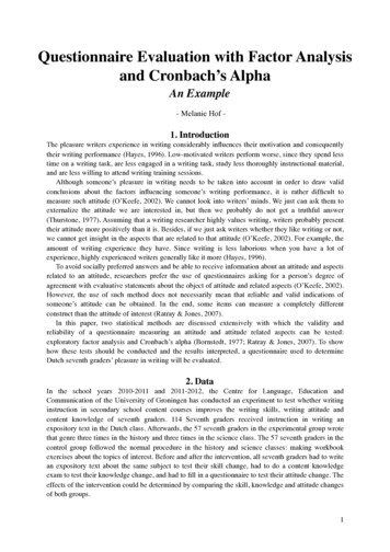
well. Hence, one’s total score on the twenty items of the questionnaire of interest should representone’s pleasure in writing correctly. Exploratory factor analysis detects the constructs - i.e. factors - thatunderlie a dataset based on the correlations between variables (in this case, questionnaire items) (Field,2009; Tabachnik & Fidell, 2001; Rietveld & Van Hout, 1993). The factors that explain the highestproportion of variance the variables share are expected to represent the underlying constructs. Incontrast to the commonly used principal component analysis, factor analysis does not have thepresumption that all variance within a dataset is shared (Costello & Osborne, 2005; Field, 2009;Tabachnik & Fidell, 2001; Rietveld & Van Hout, 1993). Since that generally is not the case either,factor analysis is assumed to be a more reliable questionnaire evaluation method than principalcomponent analysis (Costello & Osborne, 2005).3.1. Prerequisites321Sample Quantiles45In order to conduct a reliable factor analysis the sample size needs to be big enough (Costello &Osborne, 2005; Field, 2009; Tabachnik & Fidell, 2001). The smaller the sample, the bigger the chancethat the correlation coefficients between items differ from the correlation coefficients between items inother samples (Field, 2009). A common rule of thumb is that a researcher at least needs 10-15participants per item. Since the sample size in this study is 114 instead of the required 200-300, wecould conclude that a factor analysis should not be done with this data set. Yet, it largely depends onthe proportion of variance in a dataset a factor explains how large a sample needs to be. If a factorexplains lots of variance in a dataset, variables correlate highly with that factor, i.e. load highly on thatfactor. A factor with four or more loadings greater than 0.6 “is reliable regardless of samplesize.” (Field, 2009, p. 647). Fortunately, we do not have to do a factor analysis in order to determinewhether our sample size is adequate, the Kaiser-Meyer-Okin measure of sampling adequacy (KMO)can signal in advance whether the sample size is large enough to reliably extract factors (Field, 2009).The KMO “represents the ratio of the squared correlation between variables to the squared partialcorrelation between variables.” (Field, 2009, p. 647). When the KMO is near 0, it is difficult to extracta factor, since the amount of variance just two variables share (partial correlation) is relatively large incomparison with the amount of variance two variables share with other variables (correlation minuspartial correlation). When the KMO is near 1, a factor or factors can probably be extracted, since theopposite pattern is visible. Therefore,KMO “values between 0.5 and 0.7 aremediocre, values between 0.7 and 0.8 aregood, values between 0.8 and 0.9 aregreat and values above 0.9 aresuperb.” (Field, 2009. p. 647). The KMOvalue of this dataset falls within the lastcategory (KMO 0.922).Another prerequisite for factoranalysis is that the variables are measuredat an interval level (Field, 2009). A Likertscale is assumed to be an interval scale(Ratray & Jones, 2007), although the itemscores are discrete values. That hindersthe check of the next condition: the datashould be approximately normally-2-1012distributed to be able to generalize theTheoretical Quantilesresults beyond the sample (Field, 2009)and to conduct a maximum likelihoodFigure 1. Q-Q plot of the variable p06: ‘I make sure that Ifactor analysis to determine validly howhave to write as less as possible.’3
many factors underlie the dataset (see §3.3.1) (Costello & Osborne, 2005). Normality tests seem not tobe able to test normality of distribution in a set of discrete data. The normality tests signal nonnormality of distribution in this dataset by rendering p-values far lower than 0.05, although we can seea pattern of normal distribution in the Q-Q plots with a bit of fantasy. For example, the sixth item inthe questionnaire “I make sure that I have to write as less as possible.” is far from normally distributedaccording to the Shapiro-Wilk test (W 0.9136, p 1.777e-06), but does seem normally distributed inFigure 1. The exact values are centered in five groups, of which the centers are on the Q-Q line. Mostpoints are centered at the middle of the line, there are a bit less points with values of 2 or 4, and veryfew points with values of 1 or 5. Based on the Q-Q plots, I concluded that the dataset is approximatelynormally distributed, and therefore usable in a maximum likelihood factor analysis and generalizableto the population of Dutch seventh graders. If we want to generalize for a larger population, we needto conduct the same survey among other (sub)groups in the population as well (Field, 2009).The final step before a factor analysis can be conducted is generating the correlation matrix andchecking whether the variables do not correlate too highly or too lowly with other variables (Field,2009). If variables correlate too highly (r 0.8 or r -.8), “it becomes impossible to determine theunique contribution to a factor of the variables that are highly correlated.” (Field, 2009, p. 648). If avariable correlates lowly with many other variables (-0.3 r 0.3), the variable probably does notmeasure the same underlying construct as the other variables. Both the highly and lowly correlatingitems should be eliminated. As can be seen in Table 2, none of the questionnaire items correlates toohighly with other items, but some correlate too lowly with several other items. That does notnecessarily mean that the items should be eliminated: the variables with which they do not correlateenough could constitute another factor. There is one objective test to determine whether the items donot correlate too lowly: Barlett’s test. However, that test tests a very extreme case of non-correlation:all items of the questionnaire do not correlate with any other item. If the Barlett’s test gives asignificant result, we can assume that the items correlate anyhow, like in this data set: χ2 (190) 1263.862, p 7.117332e‐158. Since the Barlett’s test gives a significant result and the items correlateat most with a third of the items too lowly, items were not excluded before the factor analysis 75-0.400.561.00Table 2. Correlation matrix of the dataset. The underlined correlations are too low (-0.3 r 0.3).4
3.2. The factor analysis402Eigen values of factors683.2.1. Factor extractionAt heart of factor extraction lies complex algebra with the correlation matrix, it reaches beyond thescope of this paper to explain that comprehensively and in full detail. I refer the interested reader tochapter 6 and 7 of Statistical Techniques for the Study of Language and Language Behaviour (Rietveld& Van Hout, 1993).The algebraic matrix calculations finally end up with eigenvectors (Field, 2009; Tabachnik &Fidell, 2001; Rietveld & Van Hout, 1993). As can be seen in Figure 2, these eigenvectors are linearrepresentations of the variance variables share. The longer an eigenvector is, the more variance itexplains, the more important it is (Field, 2009). We can calculate an eigenvector’s value by countingup the loadings of each variable on the eigenvector. As demonstrated in Figure 3, just a smallproportion of the 20 eigenvectors of the correlation matrix in this study has a considerable eigenvalue:many reach 0 or have even lower values. We just want to retain the eigenvectors - or factors - thatexplain a considerable amount of the variance in the dataset, by which value do we draw the line?Statistical packages generally retain factors with eigenvalues greater than 1.0 (Costello & Osborne,2005). Yet, then there is a considerable change that too many factors are retained: in 36% of thesamples Costello and Osborne studied (2005), too many factors were retained.A more reliable and rather easy method is to look at the scree plot, as the graph in Figure 3 is called(Costello & Osborne, 2005). The factors with values above the point at which the curve flattens outshould be retained. The factors with values at the break point or below should be eliminated. Thestatistical package R helps to determine where the break point is by drawing a straight line at thatpoint. Thus, looking at Figure 3, two factors should be retained.However, the best method to determine how many factors to retain is a maximum likelihood factoranalysis, since that measure tests how well a model of a particular amount of factors accounts for thevariance within a dataset (Costello & Osborne, 2005). A high eigenvalue does not necessarily meanthat the factor explains a hugh amount of the variance in a dataset. It could explain the variance in onecluster of variables, but not in another one. That cluster probably measures another underlying factor5Figure 2. Scatterplot of two variables (x1 and x2). Thelines e1 and e2 represent the eigenvectors of thecorrelation matrix of variables x1 and x2. The eigenvalueof an eigenvector is the length of an eigenvectormeasured from one end of the oval to the other end.101520Figure 3. Screeplot of factorsunderlying the dataset.factor numberEvery point represents one factor.5
Call:factanal(x na.omit(passion), factors 1)Loadings:Factor1p01 0.767p02 0.710p03 0.786p04 -0.637p05 0.557p06 -0.542p07 0.520p08 -0.572p09 0.782p10 -0.529p11 -0.545p12 0.599p13 0.605p14 0.719p15 0.714p16 -0.558p17 0.830p18 -0.559p19 0.674p20 0.783SS loadingsProportion VarFactor18.6350.432Test of the hypothesis that 1 factor is sufficient.The chi square statistic is 336.46 on 170 degrees of freedom.The p-value is 4.89e-13Call:factanal(x na.omit(passion), factors 2, rotation "oblimin")Loadings:Factor1 Factor2p01 0.547 -0.289p02 0.747p03 0.727p040.802p05 0.625p060.641p07 0.463p08 -0.1330.558p09 0.702 -0.115p100.597p110.680p12 0.412 -0.243p13 0.7190.122p14 0.739p15 0.758p160.771p17 0.917p180.739p19 0.623p20 0.771SS loadingsProportion VarCumulative tor Correlations:Factor1 Factor2Factor11.000 -0.642Factor2 -0.6421.000Test of the hypothesis that 2 factors are sufficient.The chi square statistic is 197.76 on 151 degrees of freedom.The p-value is 0.00636Call:factanal(x na.omit(passion), factors 3, rotation "oblimin")Loadings:Factor1 Factor2 Factor3p01 0.565 -0.2630.293Factor1 Factor2 Factor3p02 0.7670.279SS loadings5.9633.5390.585p03 0.720 -0.106Proportion Var0.2980.1770.029p040.781 -0.121Cumulative Var0.2980.4750.504p05 0.600-0.134p060.6720.166p07 0.438 -0.153 -0.336p08 -0.1300.575Table 3. Output of a factor analysis in R with 1, 2 or 3 extracted factors6
or Correlations:Factor1 Factor2 Factor3Factor1 1.0000 -0.6148 -0.0385Factor2 -0.6148 1.0000 0.0596Factor3 -0.0385 0.0596 1.0000Test of the hypothesis that 3 factors are sufficient.The chi square statistic is 153.68 on 133 degrees of freedom.The p-value is 0.106Table 3. Output of a factor analysis in R with 1, 2 or 3 extracted factorswhich should not be ignored. The null hypothesis in a maximum likelihood factor analysis is that thenumber of factors fits well the dataset, when the null hypothesis is rejected a model with a largeramount of factors should be considered. As can be seen in Table 3, a model with one factor is rejectedat an α-level of 0.01, a model with two factors is rejected at an α-level of 0.05 and a model with threefactors at none of the usual α-levels (p .106). If we would set our α-level at 0.05 as common in socialscientific research (Field, 2009), a model with three factors would be the best choice. However, thethird factor seems rather unimportant, it just explains 2.9% of the variance in the dataset and is basedon just one variable p07. Variables with loadings lower than 0.3 are considered to have a nonsignificant impact on a factor, and need therefore to be ignored (Field, 2009). It seems moreappropriate to set our α-level at 0.01 and assume that two factors should be retained. The second factoraccounts for a considerable amount of the variance in the dataset: 17,7%. All variables load highly onthat factor, except for the ones that load higher on the other factor and therefore seem to make up thatone. Finally, the scree test rendered the same result.3.2.2. Factor rotationWhen several factors are extracted, the interpretation of what they represent should be based on theitems that load on them (Field, 2009). If several variables load on several factors, it becomes ratherdifficult to determine the construct they represent. Therefore, in factor analysis, the factors are rotatedtowards somevariablesExploratoryFactorAnalysisand away from some other. That process is illustrated in Figure 4. In7 thatFactor 1Factor 1Factor 2Factor 2 FigureFigure2: graphicalrepresentationof factorrotation.The left graphrepresentsrotation(right).and theThe4. Graphicalpresentationof factorrotation:orthogonalrotation(left) andorthogonaloblique rotationone representsobliquerotation.representvariablesthe loadingsof theoriginalvariablesaxesrightrepresentthe extractedfactors,the Thestarsstarsthe original(graphsource:Field,2000,onp. the439)factors. (Source for this figure: Field 2000: 439).7There are several methods to carry out rotations. SPSS offers five: varimax, quartimax,equamax, direct oblimin and promax. The first three options are orthogonal rotation; the lasttwo oblique. It depends on the situation, but mostly varimax is used in orthogonal rotation and
analysis, two factors were retained. One is represented as the x-axis, the other one as the y-axis. Thevariables (the stars) get their positions in the graph based on their correlation coefficients with bothfactors. It is rather ambiguous to which the circled variable belongs (left graph). It loads just a bit moreon factor 1. However, by rotating both factors, the ambiguity gets solved: the variable loads highly onfactor 1 and lowly on factor 2.As can be seen in Figure 4, there are two kinds of rotation. The first kind of rotation ‘orthogonalrotation’ is used, when the factors are assumed to be independent (Field, 2009; Tabachnik & Fidell,2001; Rietveld & Van Hout, 1993). The second kind of rotation ‘oblique rotation’ is used, when thefactors are assumed to correlate. Since it was assumed that all 20 items in this questionnaire measuredthe same construct, we may expect that an oblique rotation is appropriate. This can be checked afterhaving conducted the factor analysis, since statistical packages always give a correlation matrix of thefactors when you opt an oblique rotation method (oblimin or promax). Therefore, it is highlyrecommended to always do a factor analysis with oblique rotation first, even if you are quite sure thatthe factors are independent (Costello & Osborne, 2005). The factors in this study certainly correlatewith each other, although negatively: r -0.64.3.3.3. Factor interpretationIgnoring the variables that load lower than 0.3 on a factor (see §3.3.1), we can conclude based on theoutput of the factor analysis with two extracted factors (see Table 3) that the positively formulateditems in this questionnaire make up the first factor and the negatively formulated items the secondfactor. It is a rather common pattern that reverse-phrased items load on a different factor (Schmitt &Stults, 1985), since people do not express the same opinion when they have to evaluate a negativelyphrased item instead of a positively phrased one (Kamoen, Holleman & Van den Bergh, 2007). Peopletend to express their opinions more positively when a questionnaire item is phrased negatively(Kamoen, Holleman & Van den Bergh, 2007). However, it can be expected that the two factorsmeasure the same underlying construct, since they correlate considerably in a negative direction. It isafter all expected that seventh graders who score highly on the negatively phrased items (hence,dislike writing), do not score highly on the positively phrased ones.4. Cronbach’s alphaWhen the questionnaire at issue is reliable, people completely identical - at least with regard to theirpleasure in writing - should get the same score, and people completely different a completely differentscore (Field, 2009). Yet, it is rather hard and time-consuming to find two people who are fully equal orunequal. In statistics, therefore, it is assumed that a questionnaire is reliable when an individual itemor a set of some items renders the same result as the entire questionnaire.The simplest method to test the internal consistency of a questionnaire is dividing the scores aparticipant received on a questionnaire in two sets with an equal amount of scores and calculating thecorrelation between these two sets (Field, 2009). A high correlation signals a high internal consistency.Unfortunately, since the correlation coefficient can differ depending on the place at which you split thedataset, you need to split the dataset as often as the number of variables in your dataset, calculate acorrelation coefficient for all the different combinations of sets and determine the questionnaire’sreliability based on the average of all these coefficients. Cronbach came up with a faster andcomparable method to calculate a questionnaire’s reliability:α (N²M(Cov))/( s² Cov)Assumption behind this equation is that the unique variance within variables (s²) should be rathersmall in comparison with the covariance between scale items (Cov) in order to have an internalconsistent measure (Cortina, 1993).8
Reliability analysisCall: alpha(x passion)alpha average r mean0.930.423.3sd0.36Reliability if an item is dropped:alphaaverage 190.930.42p200.930.41Item statisticsnrr.corp01 114 0.77 0.76p02 114 0.68 0.67p03 114 0.77 0.76p04- 114 0.70 0.69p05 113 0.57 0.55p06- 114 0.61 0.59p07 114 0.55 0.52p08- 114 0.63 0.60p09 114 0.78 0.77p10- 114 0.59 0.57p11- 114 0.60 0.58p12 114 0.62 0.59p13 114 0.60 0.57p14 114 0.71 0.70p15 114 0.71 0.70p16- 113 0.63 0.62p17 113 0.80 0.80p18- 114 0.62 0.61p19 114 0.67 0.66p20 114 0.77 0.76mean sd3.5 1.193.9 1.073.6 1.063.3 1.293.8 0.903.0 1.193.4 0.822.6 1.183.6 0.982.5 1.233.1 1.263.0 1.003.4 1.083.7 1.013.8 0.953.4 1.123.8 0.852.6 1.173.2 1.063.8 0.94Table 4. Output of a Cronbach’s alpha analysis in R4.1. PrerequisiteBefore the Cronbach’s alpha of a questionnaire can be determined, the scoring of reverse-phraseditems of a questionnaire needs to be reversed (Field, 2009). Hence, a score of 5 on a negativelyformulated item in this questionnaire should be rescored in 1, a score of 4 in 2, et cetera. Assumingthat a seventh grader who really likes writing strongly agrees with the statement ‘I like writing’ andstrongly disagrees with the statement ‘I hate writing’, item scores can differ substantially betweenstudents as long as the scores of the reverse-phrased items are not reversed. Given that covariancesbetween such scores are negative, the use of reverse-phrased items will finally lead to a lower andconsequently incorrect Cronbach’s alpha, since the top half of the Cronbach’s alpha equationincorporates the average of all covariances between items. Fortunately, R reverses scoresautomatically. Since reverse-phrased items load negatively on an underlying factor, R detects themeasily by determining that underlying factor.4.2. Cronbach’s alpha analysisGenerally, a questionnaire with an α of 0.8 is considered reliable (Field, 2009). Hence, thisquestionnaire certainly is reliable, since the α is 0.93 (see Table 4). The resulted α should yet beinterpreted with caution. Since the amount of items in a questionnaire is taken into account in theequation, a hugh amount of variables can upgrade the α (Cortina, 1993; Field, 2009). For example, ifwe do a reliability analysis for just the items making up the first factor in our research, we get the sameα, but the average correlation is 0.49 instead of 0.43. How hugh the alpha should be for a dataset witha particular amount of items is still a point of discussion (Cortina, 1993). Cortina (1993) recommendsto determine the adequacy of a measure on the level of precision needed. If you want to make a finedistinction in the level of pleasure in writing someone has, a more reliable measure is needed than ifyou want to make a rough distinction. However, since the α of this questionnaire is far higher than 0.8,we can assume that it is reliable (Field, 2009).9
Besides, a hugh Cronbach’s alpha should not be interpreted as a signal of unidimensionality (Cortina,1993; Field, 2009). Since α is a measure of the strength of a factor when there is just one factorunderlying the dataset, many researchers assume that a dataset is unidimensional when the α is ratherhigh. Yet, the α of this dataset is rather high as well, although the factor analysis revealed that thedataset is not unidimensional. Thus, if you want to measure with Cronbach’s alpha the strength of afactor or factors underlying a dataset, Cronbach’s alpha should be applied to all the factors extractedduring a previous factor analysis (Field, 2009). Our factors turn out to be quite strong: the α of thefactor made up of the positively phrased items is 0.93, the α of the factor made up of the negativelyphrased items is 0.86.The final step in the interpretation of the output of a Cronbach’s alpha analysis is determining howeach item individually contributes to the reliability of the questionnaire (Field, 2009). As can be seenin Table 4, R also renders the values of the α, when one of the items is deleted. If the α increases a lotwhen a particular item is deleted, one should consider deletion. The same counts for items whichdecrease the average correlation coefficient a lot, or correlate lower than 0.3 with the total score of thequestionnaire (see the values under r and r.cor in Table 4; r.cor is the item total correlation correctedfor item overlap and scale correlation). In this questionnaire, all items positively contribute to thereliability of the questionnaire. The α remains the same when an item is deleted, the average r almostthe same, and the correlations between the total score and the item score are moderate to high.5. ConclusionThe evaluated questionnaire seems reliable and construct valid. The items measure the sameunderlying construct. The extraction of two factors in the factor analysis just seems to be aconseq
If a factor explains lots of variance in a dataset, variables correlate highly with that factor, i.e. load highly on that factor. A factor with four or more loadings greater than 0.6 "is reliable regardless of sample size." (Field, 2009, p. 647). Fortunately, we do not have to do a factor analysis in order to determine