Transcription
Journal of Mathematical Finance, 2018, 8, 161-177http://www.scirp.org/journal/jmfISSN Online: 2162-2442ISSN Print: 2162-2434A Linear Regression Approach for DeterminingOption Pricing for Currency-Rate DiffusionModel with Dependent Stochastic Volatility,Stochastic Interest Rate, and Return ProcessesRaj JagannathanDepartment of Management Sciences, Tippie College of Business, The University of Iowa, Iowa City, USAHow to cite this paper: Jagannathan, R.(2018) A Linear Regression Approach forDetermining Option Pricing for Currency-Rate Diffusion Model with DependentStochastic Volatility, Stochastic InterestRate, and Return Processes. Journal ofMathematical Finance, 8, ived: August 14, 2017Accepted: February 25, 2018Published: February 28, 2018Copyright 2018 by author andScientific Research Publishing Inc.This work is licensed under the CreativeCommons Attribution InternationalLicense (CC BY en AccessAbstractA three-factor exchange-rate diffusion model that includes three stochastically-dependent Brownian motion processes, namely, the domestic interest rateprocess, volatility process and return process is considered. A linear regression approach that derives explicit expressions for the distribution functionof log return of foreign exchange rate is derived. Subsequently, a closedform workable formula for the call option price that has an algebraic expression similar to a Black-Scholes model, which facilitates easier study, isdiscussed.KeywordsOption Pricing, Interest-Rate Parity Condition, Black-Scholes Model, LinearRegression Approach, Spot Option, Ito Calculus1. IntroductionA foreign exchange rate depends on the supply and demand dynamics of a currency. The exchange rate is a function of trade balance, the interest rate differential and differential inflation expectations between the two countries [1] [2].Let S(u), u 0 exchange rate process over the time interval: u 0 , whereu number of domestic currency units, e.g., , per unit of foreign currency -price of foreign currency.As interest rate rD ( u ) increases, appreciates because investors prefer -denominated bonds. Assuming a frictionless, arbitrage-free continuous-timeeconomy in [1], we define a diffusion process model for S(u). In addition, usingDOI: 10.4236/jmf.2018.81013 Feb. 28, 2018161Journal of Mathematical Finance
R. Jagannathaninterest-rate parity condition we haveh ( rD ( u ) rF ( u ) )duS ( h ) S0 e 0, see [1].In the following section, the formula for valuations of currency spot options isconsidered, where we obtain a closed form formula for the call option price thathas a simple algebraic expression, which is similar to the call option price expression of a Black-Scholes model, making it much easier to compute its valueand study. As in [2], we can define an implied volatility function and derive itsskewness property.Subsequently, the proposed three-factor exchange-rate diffusion model isdiscussed, such that the stochastic volatility process and the stochastic domesticinterest rate process each have a stochastically dependent Brownian motion return process.In the next section, a linear regression approach that derives explicit expres-sions for the distribution function of ln S ( s ) is treated.Foreign exchange rate option modeling is the subject of several well-knownpapers and in chapters within [3] [4] [5] [6]. Leveraging Heston’s model [4] forthis application would introduce complexity due to the need to numerically integrate conditional characteristic functions obtained as solutions of nonlinearpdf to derive the call option prices. An equivalent two-factor Black-Derman-Toymodel [2] can be formulated with introduction of H(u).The method suggested in this paper results in Black-Scholes type formula forcall option pricing, which is easily computable.Finally, we provide concluding remarks and suggestions for future direction.2. Currency Spot OptionGiven the spot rate S ( 0 ) s0 , consider the present value of option s C * ( s0 , K ,*) E0 exp rD ( u ) du * S ( s ) K 0 (where K is the known strike price and( rD ( u ) , u 0 ))(1)is a mean-reverting sto-chastic process given in (2) below. S ( s ) is the value of the exchange rate at theoption’s maturity price. The option to purchase foreign currency over the counter can be exercised when S(s) the strike price exchange rate K.3. A Diffusion Process ModelA continuous-time risk-adjusted and risk-neutral exchange rate model, under aMartingale Measure Q, is defined below as a diffusion process (2), mean-revertingstochastic processes: Volatility{H ( u ) , u 0}(3) and domestic interest raterD ( t ) process (4), and foreign interest rate rF is a known constant.dS ( u ) S (u )DOI: 10.4236/jmf.2018.81013162 H 2 (u ) ( rD ( u ) rF ) du ( H ( u ) υ ) dB1 ( u )2 (2)Journal of Mathematical Finance
R. JagannathandH ( u ) α ( H ( u ) θ ) du η dV1 ( u ) , θ ,η 0, α 0(3)drD ( u ) β ( rD ( u ) λ ) du ζ dV2 ( u ) , λ , ζ 0, β 0(4) υ2 d ln S ( u ) rD ( u ) rF du ( H ( u ) υ ) dB1 ( u )2 (5)Equation (5) is obtained from Equation (2) by the application of Ito calculus [7].Assumption:V1 ( t ) ρ B1 ( t ) δ C ( t ) , where δ 1 ρ 2 and B1 ( t ) and C ( t ) are in dependent Brownian processes.V2 ( t ) ρ1 B1 ( t ) δ1C1 ( t ) , where δ 11 ρ12and B1 ( t ) and C1 ( t ) are independent Brownian processes.(6)From the assumption above, the return processes V j ( u ) , u 0, j 1, 2 arecorrelated with B1 ( u ) and that V j ( t ) , j 1, 2 are standard Brownian motionprocesses.Then it follows, see [2] [3], that the distributions of H ( u ) and rD ( u ) areGaussian processes.Alternatively, H ( u ) and rD ( u ) may be expressed as:uH ( u ) q ( u ) ψ ( t ) dV1 ( t ).0u H ( u ) q ( u ) ψ ( t ) ρ dB1 ( t ) δ dC ( t ) .(7)0(E ( H ( u ) ) q ( u ) κ e α u θ 1 e α u) θ (κ θ ) e α u , α 0,where θ is the long-term mean and where H ( 0 ) κ .var ( H ( u ) ) σ H2u 1 e 2α u 2α uψ 2 ( t ) dt 2 2α te dt η 2 η 00 µ So P ( H ( u ) 0 ) Φ H σH (8)Remark 1:From (8), choosing θ 0 and that is small in value, we can makeP ( H ( u ) 0 ) negligible.If, alternatively, we assume that { H ( u ) , u 0} has a square root process [8],then the random variable H(u) distribution is non-central χ 2 (.) . For simplicitywe chose the mean-reverting process model (3).()E ( rD ( u ) ) q1 ( u ) κ1e β u λ 1 e β u λ (κ1 λ ) e β u , β 0 u var ( rD ( u ) ) ψ 12 ( t ) du 0 where ψ 1 ( u ) ζ e β u , u 0 and rD ( 0 ) κ1u rD ( u ) q1 ( u ) ψ 1 ( t ) ρ1dB1 ( t ) δ1dC1 ( t ) (9)0DOI: 10.4236/jmf.2018.81013163Journal of Mathematical Finance
R. JagannathanAssuming rD ( 0 ) κ1 , and ψ 1 ( t ) θ e β t , θ , β 0, 0 t u()q1 ( u ) κ1e β u λ 1 e β u λ (κ1 λ ) e β usQ1 ( s ) ( κ1 λ ) q1 ( u ) du 1 e β sβ0(10) λsThe Brownian motion processes V1 ( u ) and B1 ( u ) are as follows:V1 ( u ) ρ B1 ( u ) δ C1 ( u ) , where δ 1 ρ2(11)In addition, the Brownian motion processes B1 ( u ) and C1 ( u ) under Q areindependent.Remark 2:H ( u ) , u 0 : the volatility process.It follows from [2] that the distribution of H ( u ) is:η H (u ) N q (u ) ,1 e 2α u2α ()12 , 0 u s. (12)Alternatively, H ( u ) may be expressed asuH ( u ) q ( u ) ψ ( t ) dV1 ( t )0u q ( u ) ψ ( t ) ρ dB1 ( t ) δ dC ( t ) (13)0where δ 1 ρ2and ψ ( u ) η e α u , η , α 0 .See [9] for a similar assumption. See also [2] and [3].Note that B1 ( s ) has a normal distribution with mean 0 and variance s, soB1 ( s ) can be written as B1 ( s ) Z ( s ) s , where Z ( s ) is a standard normalvariable. Then ln X ( s ) can be written as a quadratic function ofB1 ( s ) Z (s), s 0 plus a residual term ε ( s ) . {See Proposition 1 below}.sdξ dC ( t ) , 0 t u , 0 u s , we define a volatility processFor V (ξ ) Vu u ψ ( t ) dC ( t ), 0 u s . 0( 1 s η 2 1 e 2α uDefine σ (V ( s ) ) s 0 2α ) du 12 V , as the average standarddeviation in the case of uncorrelated Brownian motion process{C ( u ) , 0 u s} ξ[See [10], p. 182].Proposition 1:urD ( u ) q1 ( u ) ψ 1 ( t ) ρ1dB1 ( t ) δ1dC1 ( t ) ;0sssu0000 rD ( u ) du q1 ( u ) du du ψ 1 ( t ) ρ1dB1 ( t ) δ1dC1 ( t ) DOI: 10.4236/jmf.2018.81013 Q1 ( s ) ρ1 B1 ( s ) ( G1 ( s ) χ1 ( s ) ) δ1V1 e3 ( s ) .164(14)Journal of Mathematical Finance
R. Jagannathanwhere(1 e ) λ ss β sQ1 ( s ) q1 ( u ) du ( κ1 λ )0(β)js ζ 1 e β t ζ (β s)j 1 dtG (s) 1) ( ββ j 1 j ! j0 χ (s) (15)ζ β j s j 1j 1 ( 1) β j 1 ( j 1)! j sProof: See Appendix B.We consider a mean-reverting Gaussian process model (2), the volatility stochastic processes { H ( u ) , 0 u s} and the processes, V1 ( u ) and B1 ( u ) in(3) to be correlated; where V1 ( u ) is a standard Brownian motion returnprocess. In addition, in (3), we define the volatility H ( u ) ε R as a mean reverting Gaussian process with θ as its long-term mean.Assumption 1:V1 ( t ) ρ1 B1 ( t ) δ1C ( t ) , where δ1 1 ρ12(16)In (4), we define the domestic interest rate process rD ( u ) as a mean reverting Gaussian process with λ as its long-term mean. The process{rD ( u ) , 0 u s} is such that the return process V2 ( u ) is a correlated standard Brownian motion process to B1 ( u ) . The foreign interest rate rF ( u ) is aconstant rfAssumption 2:It follows from [2] that the distribution of rD ( u ) : ζrD ( u ) N q1 ( u ) ,1 e 2 β u 2β ()12 , 0 u s. (17)Now we use the results obtained in Proposition 1 to derive an explicit expression forsS (u ) d ln ln S ( s ) ln S00Proposition 2:s d ln S ( u )0 s ( rD ( u ) rF ) du 0υ22ss υ θ q0 ( u ) dB1 ( u )(18)0s u ψ ( t ) ( ρ dB1 ( t ) δ dC ( t ) ) dB1 ( u ) ;0 0 Remark 3:From the expression fors rD ( u ) du Q1 ( s ) ρ1B1 ( s ) ( G1 ( s ) χ1 ( s ) ) δ1V1 . the stochastic terms0DOI: 10.4236/jmf.2018.81013165Journal of Mathematical Finance
R. Jagannathanρ1 B1 ( s ) ( G1 ( s ) χ1 ( s ) ) modifies n ( s ) and the constant term Q1 ( s ) δ1V1modifies p* ( s, h ) with the addition of ρ1 B1 ( s ) ( G1 ( s ) χ1 ( s ) ) and the constant terms Q1 ( s ) δ1V1 modifies p* ( s, h ) with the addition of Q1 ( s ) δ1V1 .Then, using the results in [2], Proposition 1 and those in Appendix A andAppendix B we have:ln S ( s ) ln s0 υ22s rF s (υ θ ) B1 ( s ) γ 1 ( s ) B1 ( s ) e1 ( s ) B2 ( s ) s γ 2 ( s ) ρ 1 e2 ( s ) Q1 ( s ) 22 (19) ρ1 B1 ( s ) ( G1 ( s ) χ1 ( s ) ) δ1V1Y1 e3 ( s ) Z 2 (s)m(s)2 Z ( s ) n ( s ) p ( s ) ε ( s ) U ( s, ξ ) ε ( s )Therefore,U ( s, ξ ) Z 2 ( s )m(s)2 Z (s) n(s) p (s),m ( s ) ργ 2 ( s ) s;()n ( s ) (υ θ δ V ) γ 1 ( s ) γ 3 ( s ) ρ1 ( G1 ( s ) χ1 ( s ) ) δ1V1 s ; Remark 4:Note that n ( s ) in this paper is an updated version from the n ( s ) in [2],due to our treatment of a stochastic interest rate:s rD ( u ) du01sp ( s ) ln s0 υ 2 s ργ 2 ( s ) ε ( s ) Q1 ( s ) rF s;22s η 2 1 e 2α u () duσ 2 (V ( s ) ) 2α 0 (1 s η 1 e s 0 2α 21η s2 2α u) 2du( 2α s (1 e )) V 2α s4α 22,In the case of C ( u ) , u 0 .σ 2 (V1 ( s ) ) 1ζs2( 2β s (1 e )) V 2 β s4β 221, where C1 ( u ) , u 0(20)m ( s ) ργ 2 ( s ) s;n ( s ) (υ θ δ V ) γ 2 ( s ) λ γ 3 ( s ) ω2 ρ1 ( G1 ( s ) χ1 ( s ) ) s (21)1sp ( s ) ln S0 υ 2 s ργ 2 ( s ) ε ( s ) Q1 ( s ) rF s δ1V122ε ( s ) e1 ( s ) e2 ( s ) e3 ( s ) whereDOI: 10.4236/jmf.2018.81013166Journal of Mathematical Finance
R. Jagannathan Q1 ( s )sq1 ( u ) du 01sγ1 ( s ) q0 ( u ) dus 0(κ1 λ ) (1 e β s )1β1(κ θ ) (1 e α s )αs2η s u2ηγ 2 (s) ψ ( t ) dtdu 2 s 00s2 ((2η α s 1 eα2s2 α s))s λ s;;(22)(1 e ) du α uα0. 1 e 2α s 1 e α 2 Var ( e1 ( s ) ) ( κ θ ) ; 2α α s 2 η 2 s η 2 η s η Var ( e2 ( s ) ) 2 1 e 2α s 2 1 e α s 2αα4αα ()()2Var ( e3 ( s ) ) is provided in (B1)Cov ( ei ( s ) , e j i, j 1, 2,3, i j( s ) ) 0; Case 1: ρ 0 ;s d ln S ( u )0 s ( rD ( u ) rF ) du υ2sss ( λ1 q1 ( u ) ) du υ θ q0 ( u ) dB1 ( u )200s u ψ ( t ) ( ρ dB1 ( t ) δ C ( t ) ) dB1 ( u ) ψ 1 ( t ) ( ρ1dB1 ( u ) δ1dC1 ( u ) ) ;0 00 0sLet S ( 0 ) s0ln S ( s ) ln S0 υ22s rF s (υ θ δ V ) B1 ( s ) B2 ( s ) s γ 1 ( s ) B1 ( s ) e1 ( s ) γ 2 ( s ) ρ 1 e2 ( s ) 2 2 Q1 ( s ) ρ1 B1 ( s ) ( G1 ( s ) χ1 ( s ) ) δ1V1 e3 ( s ) .Let ln S ( s ) Z 2 ( s )m(s) Z ( s ) n ( s ) p ( s ) ε ( s ) U ( s, ξ ) ε ( s ) .2Assumption 3: U ( s, ξ ) and ε ( s ) are independent random variables.Assumption 4: n 2 ( s, ξ ) 2m ( s ) ( p ( s, h ) ω ) 0 .Assumption 5: m ( s ) 0 and m ( s ) 1 .If Assumptions (4) and (5) hold, then the conditional risk-neutral distributionof ln S ( s ) is:Proposition 3:1 Fln S ( s ) (ω , h )1 Φ ( z1 ( h ) ) Φ ( z2 ( h ) ) , ω ω ( ρ , h, ξ ) P ( ln S ( s ) ω ε ( s ) h) 1, ω ω ( ρ , h, ξ )DOI: 10.4236/jmf.2018.81013167Journal of Mathematical Finance
R. JagannathanΦ ( z1 ( h ) ) Φ ( z2 ( h ) ) , ω ω ( ρ , h, ξ )P ( ln S ( s ) ω ε ( s ) h) Fln S ( s ) (ω , h ) 0, ω ω ( ρ , h.ξ )(23)where z z 1 ( h, ξ ) , z 2 ( h , ξ )ω* ( ρ , h ) h p (s) n ( s ) n 2 ( s, ξ ) 2m ( s ) ( p ( s ) h ω )m(s)(24)n (s)22m ( s )()If n 2 ( s, ξ ) 2m ( s ) p ( s ) h ω * 0 , then the roots of the equation definedin (24) are equal so that z1 z2 z (ξ ) n ( s, ξ )m(s), then there exists a valueω ( ρ , h, ξ ) such that()P ln S ( s ) ω ( ρ , h ) ε ( s ) h, V 2 ( s ) 1.ξ In other words, ω * ( ρ , h, ξ ) is the lowest value for the conditional randomvariable ln ( S ( s ) ) .Remark 5:Since we know the CDF of lnS(s) we can estimate the parameters of the underlying model (2)-(5).Case 2: Conditional Risk-neutral Distribution function of ε ( s ) h , V ( s ) ξ ) , m ( s ) 0 . Suppose ρ 0 , Conditional risk-neutral( ln S ( s ) distribution of ln S ( s ) ( ε ( s ) h , V 2 ( s ) ξ ) is as follows:1 Fln S ( s ) ξ (ω , h ) P ( ln S ( s ) ω ε ( s ) h, V ( s ) ξ ) Φ ( z2 ( h ) ) Φ ( z1 ( h ) ) , ω ω ( ρ , h, ξ ) 0, ω ω ( ρ , h, ξ )1 Φ ( z2 ( h ) ) Φ ( z1 ( h ) ) , ω ω ( ρ , h, ξ ) Fln S ( s ) ξ (ω , h ) 1, ω ω ( ρ , h )wherez z 1 ( h, ξ ) , z 2 ( h , ξ ) n ( s, ξ ) n 2 ( s, ξ ) 2m ( s ) ( p ( s ) h ω )m(s)Example 1drD ( 0 ) κ1 ;u ) β ( rD ( u ) λ ) du ζ dV2 ( u ) , λ , ζ 0, β 0, rD ( drD ( u ) 0.3 ( rD ( u ) 0.02 ) du 0.04dV2 ( u ) , rD ( 0 ) 0.03;dH ( u ) α ( H ( u ) θ ) du ηV1 ( u ) , H ( 0 ) κ ;dH ( u ) ( H ( u ) 0.1) du 0.3V1 ( u ) , H ( 0 ) 0.6DOI: 10.4236/jmf.2018.81013168Journal of Mathematical Finance
R. JagannathanrD ( u ) :βλζrD ( 0 ) κ1ρ10.30.20.40.030.6H (u ) :αθηρκrf10.10.3 0.80.60.8Thenp* ( s, h ) p ( s ) h Q1 ( s ) ln s ( 0 ) ln K ρ1Y1Remark 6:From the expression fors rD ( u ) du Q1 ( s ) ρ1B1 ( s ) ( G1 ( s ) χ1 ( s ) ) δ1V1.0the stochastic terms ρ1 B1 ( s ) ( G1 ( s ) χ1 ( s ) ) modify the term n ( s ) and theconstant terms Q1 ( s ) δ1V1 modifies p* ( s, h ) with the addition ofQ1 ( s ) δ1V1 .Proof:Apply a proof similar to the one in Appendix A of [2] using the result forr D ( u ) du in Appendix B of the current paper. See also Proposition 4.0Remark 7:Assume ρ 0 , which implies that m ( s ) 0 .If Assumption (3) holds then the conditional risk-neutral distribution ofln ε ( s ) h , V ( s ) ξ } is:{ S ( s ) s1 Fln S ( s ) (ω , h )1 Φ ( z1 ( h ) ) Φ ( z2 ( h ) ) , ω ω ( ρ , h, ξ ) P ( ln S ( s ) ω ε ( s ) h) 1, ω ω ( ρ , h, ξ ) Fln S ( s ) ξΦ ( z1 ( h ) ) Φ ( z2 ( h ) ) , ω ω ( ρ , h, ξ )P ( ln S ( s ) ω ε ( s ) h) (ω , h ) 0, ω ω ( ρ , h, ξ )(25)where z z 1 ( h, ξ ) , z 2 ( h , ξ )ω ( ρ, h) h p (s) * n ( s ) n 2 ( s, ξ ) 2m ( s ) ( p ( s ) h ω )m(s)n2 ( s )(26)2m ( s )If n 2 ( s, ξ ) 2m ( s ) ( p ( s ) h ω * ) 0 , then the roots of the equation definedin (26) are equal so that z1 z2 z (ξ ) DOI: 10.4236/jmf.2018.81013169n ( s, ξ )m(s), then there exists a valueJournal of Mathematical Finance
R. Jagannathanω ( ρ , h, ξ ) such that P ( ln S ( s ) ω ( ρ , h ) ε ( s ) h, V 2 ( s ) ξ) 1.In other words, ω * ( ρ , h, ξ ) is the lowest value of the conditional randomvariable{ln S ( s ) ε ( s ) hσ ( )} .ε sCall option price: s c* ( s, S ( s ) , K , S ( 0 ) ) E0Q exp rD ( u ) du ln S ( s ) ln K 0 Proposition 4:C ( s0 , K , r ,η , h, ρ 0 ) s rD ( u )du E e 0S (s) K ) ε (s) h ( 0, for ln K ω ( ρ , h ) ; z ( h ) (1 m ( s ) ) n ( s ) 1 z2 ( h ) (1 m ( s ) ) n ( s ) s0 1 Φ Φ 1212 1 m ( s ) (1 m ( s ) )(1 m ( s ) ) s rd ( u )du n 2 ( s ) exp p* ( s, h ) ln S ( s ) ln K KE e 0 2 (1 m ( s ) ) Q0where from Proposition 1s rD ( u ) du Q1 ( s ) ρ1B1 ( s ) ( G1 ( s ) χ1 ( s ) ) δ1V1.0See Appendix B.p* ( s, h ) { p ( s ) ε ( s ) h} ln s0 ln K Q1 ( s ) δ1V1 Remark 8:Given the formula fors rD ( u ) du Q1 ( s ) ρ1B1 ( s ) ( G1 ( s ) χ1 ( s ) ) δ1V1 ,the stochastic expression0ρ1 B1 ( s ) ( G1 ( s ) χ1 ( s ) ) modifies the function n ( s ) and the constant termsQ1 ( s ) δ1V1 , modifies p* ( s, h ) with the addition of Q1 ( s ) δ1V1 . s rD ( u )du K e 0 ln S ( s ) ln K z2 h z 1h{()}K exp ( Q1 ( s ) δ1V1 ) G1 ( s ) χ ( s ) ρ1 z s e z 2 dzz2 h K z eA( s ) A1 ( s ) z z 222(27)dz;1hLetA1 ( s ) z ρ1 ( G1 ( s ) χ1 ( s ) ) B1 ( s ) ρ1 ( G1 ( s ) χ1 ( s ) ) z s ;A ( s ) Q1 ( s ) δ1V1 A ( s ) A1 ( s ) z DOI: 10.4236/jmf.2018.81013170A2 ( s )2z2 z A1 ( s ) 2 2 A ( s ) 1;28(28)Journal of Mathematical Finance
R. JagannathanThenz2 hK z eA( s ) A1( s ) z z 2 2dz1 A2 ( s ) Φ z2 h A1 ( s ) 2 Φ z1h A1 ( s ) 2 exp A ( s ) 1 ; 8 Hedge Ratio: C * (.) s0 z ( h ) (1 m ( s ) ) n ( s ) z ( h ) (1 m ( s ) ) n ( s ) 1 2 Φ 1 Φ 1212 1 m(s) (1 m ( s ) )(1 m ( s ) ) n2 ( s ) exp p* ( s, h ) , ln K ω * ( ρ , h ) ; 21ms ( ( ) ) 0, ln K ω * ( ρ , h ) ; -Neutral PortfolioDelta-Neutral PortfolioConsider the following portfolio that includes a short position of one European call and a long position of delta units of the domestic currency.The portfolio of delta-neutral positions is defined as:P s0 c* Hedge ratio ( P ) 0We obtain below Conditional Risk-neutral Distribution function ofs) ε (s)( ln S ( ξ ), m(s) 0hσ ε ,V ( s )(29)by considering the cases of: h 1, 0 and 1We use a discrete approximation (see [2], (28)).Suppose ρ 0 , which implies m ( s ) 0 .Again, we consider the Equations (1)-(4) to define Example 1 below.dS ( u ) S (u ) H 2 (u ) rD ( u ) rF du ( H ( u ) υ ) dB1 ( u ) ;2 (30)dH ( u ) α ( H ( u ) θ ) du η dV1 ( u ) , θ ,η 0, α 0;(31)drD ( u ) β ( rD ( u ) λ ) du ζ dV2 ( u ) , λ , ζ 0, β 0;(32) υ2 d ln S ( u ) rD ( u ) rF du ( H ( u ) υ ) dB1 ( u ) ;2 (33)LetdrD ( u ) β ( rD ( u ) λ ) du ζ dV2 ( u ) , λ , ς 0, β 0, rD ( 0 ) κ1 ;drD ( u ) 0.3 ( rD ( u ) 0.02 ) du 0.04dV2 ( u ) , rD ( 0 ) 0.03;dH ( u ) α ( H ( u ) θ ) du ηV1 ( u ) , H ( 0 ) κ ;dH ( u ) ( H ( u ) 0.1) du 0.3V1 ( u ) , H ( 0 ) 0.6DOI: 10.4236/jmf.2018.81013171Journal of Mathematical Finance
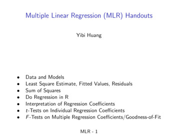
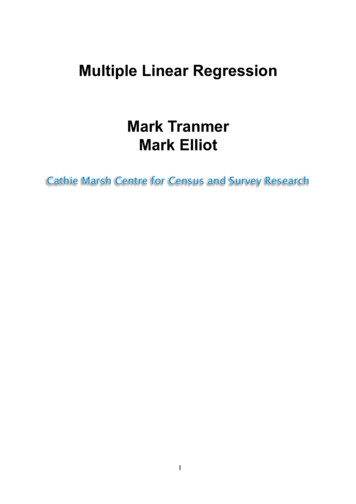
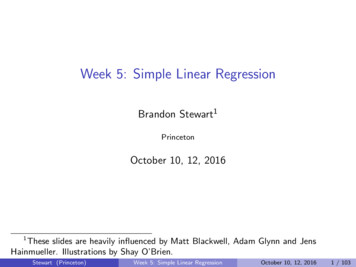
R. JagannathanThen, H ( u ) :υαηθρκδsH ( 0)0.0810.20.1 0.80.10.60.50.06And rD ( u ) :βθ1λδ1ζρ1rf0.30.20.10.50.04340.06If Assumption (2) holds then the unconditional risk-neutral distribution of()ln S ( s ) ε ( s ) h , V 2 ( s ) ξ and U ( s, ξ ) are independent random variables.Then Figure 1 depicts the unconditional risk-neutral distribution ofP {ln S ( s ) u h} Fln( S ( s ) ( u h ) .Remark 9:Future movement of values of risk-free interest rate and volatility are uncertain and as they increase, they affect call option values as depicted in the aboveFigure 2, Figure 3 ([5], p. 204). Sudden changes in their values may occur because of economic shock. See the models suggested in [11] [12].Unconditional Risk Neutral CumulativeDistribution Function of ln(S(s))0.50.40.30.2Unconditional RiskNeutral e 1. Unconditional risk-neutral CDF of lnS(s), strike price (cents) kfrom 1.1 to 16.2.Unconditional Call Option Price4035302520Unconditional CallOption Price .52223.5250Figure 2. Unconditional call option price with strike price k (cents) from1.1 to 26.DOI: 10.4236/jmf.2018.81013172Journal of Mathematical Finance
R. JagannathanUnconditional Hedge Ratio350300250200Unconditional HedgeRatio150100501.1357911131517192123250Figure 3. Unconditional hedge ratio with strike price k (cents) from 1.1to 26.4. ConclusionWe define a three-factor exchange-rate diffusion model with 1) stochastic volatility process, 2) stochastic domestic interest rate process, and 3) return processwhich are Brownian motion return processes that are stochastically dependent.Further generalization is possible with the assumption of domestic and foreignstochastic interest rate processes which are subject to economic shocks [11] [12].The results are applicable to bond option models ([5], p. 783).References[1]Krugman, P.R. and Obstfeld, M. (2000) International Economics. 3rd Edition, Addison Wesley, Boston, 360-362.[2]Jagannathan, R. (2016) A Linear Regression Approach to Two-Factor Option Pricing Model. Journal of Math Finance, 6, 317-337.[3]Vasicek, O. (1977) An Equilibrium Characterization of the Term Structure. JournalFinancial Economics, 5, 177-188. ton, S. (1993) A Closed-Form Solution for Options with Stochastic Volatilitywith Applications to Bond and Currency Options. Review of Financial Studies, 6,327-344. https://doi.org/10.1093/rfs/6.2.327[5]Hull, J.C. (2009) Options, Futures and Derivatives. Pearson, Prentice Hall, UpperSaddle River.[6]Garman M.B. and Kohlhagen, S.W. (1983) Foreign Exchange Option Values. Journal of International Money and Finance, 2, 1-1[7]Oksendal, B. (2003) Stochastic Differential Equations—An Introduction with Applications. Springer, New York.[8]Cox, J.C., Ingersoll, J.E. and Ross, S.A. (1985) A Theory of the Term Structure ofInterest Rates. Econometrics, 53, 385-407. https://doi.org/10.2307/1911242[9]Trolle, A.B. and Schwarz, E.S. (2009) A General Stochastic Volatility Model for thePricing of the Interest Rate Derivatives. The Review of Financial Studies, 22,2007-2057. https://doi.org/10.1093/rfs/hhn040[10] Duffie, D. (1996) Dynamic Asset Pricing Theory. 2nd Edition, Princeton UniversityPress, Princeton.[11] Merton, R.C. (1976) Option Pricing When the Underlying Stock Returns Are DisDOI: 10.4236/jmf.2018.81013173Journal of Mathematical Finance
R. Jagannathancontinuous. Journal of Financial Economics, 3, 125-144.[12] Jagannathan, R. (2008) A Class of Asset Pricing Models Governed by SubordinatedProcesses That Signal Economic Shocks. Journal of Economic Dynamics and Control, 32, 3820-3846. https://doi.org/10.1016/j.jedc.2008.04.004[13] Bakshi, G., Cao, C. and Chen, Z. (1997) Empirical Performance of Alternative Option Pricing Models. The Review of Financial Studies, 52, .tb02749.x[14] Wilks, S.S. (1962) Mathematical Statistics. John Wiley, Hoboken.DOI: 10.4236/jmf.2018.81013174Journal of Mathematical Finance
R. JagannathanAppendix A( () )s 1 eα s α2 s u2 s 1 e α u2duψtdtηduη ()αs 2 0 0s 2 0 αs2γ 2 (s) ((αs2 α s 1 eηs2α22 s uγ 2 ( s ) 2 du ψ ( t ) dts 0 0is the regression coefficient. ))2s2 e2 ( s ).s u (ψ ( t ) γ 2 ( s ) ) dB1 ( t ) dB1 ( u ).0 0 E ( e2 ( s ) ) 0; E ( e1 ( s ) ) 0, Cov ( e1 ( s ) , e2 ( s ) ) 0Var ( e2 ( s ) ) su00 du (ψ ( t ) γ 2 ( s ) )22s2dt (2A1)s u22 ψ ( t ) dtdu γ 2 ( s )0 0Then the regression equation iss ψ ** ( s ) γ 2 ( s ) B12 ( s ) 2 e2 ( s ) ;2 Assumption 6:(e2 ( s ) N 0,Var1 2 ( e2 ( s ) ))(2A2)(Approximately)Note that Cov ( e1 ( s ) , e2 ( s ) ) 0 and((2A3))e1 ( s ) N 0,Var1 2 ( e2 ( s ) ) .( Var ( e1 ( s ) ) Var ( e2 ( s ) )1/2Assumption 7:) Var ( e ( s )) Var ( e ( s ))1(2ε (s) e1 ( s ) e2 ( s ) N 0, (Var ( e1 ( s ) ) Var ( e2 ( s ) ) )12)(Approximately)(2A4)Proof of Proposition 1:s 0 S ( u ) du {rd ( u ) r d ln s0u(} υ2 2f) υ θ q0 ( u ) ψ ( t ) ( ρ dB1 ( t ) δ dC1 ( t ) ) dB1 ( u );0{}1ln S s ln s0 rd ( u ) r f du υ 2 s (υ θ ) B1 ( s )2 B2 ( s ) s γ 1 ( s ) B1 ( s ) e1 ( s ) γ 2 ( s ) ρ 1 e2 ( s ) δ VB1 ( s ) 22 2s B (s) s 1 ln s0 rd ( u ) du υ 2 s (υ θ ) ρ 1 222 0 B 2 (s) s γ 1 ( s ) B1 ( s ) e1 ( s ) δ VB1 ( s ) ρ γ 2 ( s ) 1 e2 ( s ) . 2 2 DOI: 10.4236/jmf.2018.81013175Journal of Mathematical Finance
R. JagannathanAppendix A from [2]sus000B1 ( u ) ψ ( t ) dB1 ( t ) γ 2 ( s ) B1 ( u ) dB1 ( u ) e2 ( s ) d s γ 2 ( s ) B12 ( s ) e2 ( s )2 where2 s u2 s 1 e α u du ψ ( t ) d tηdu2 s 0 0s 2 0 α γ 2 (s)( () )((αss 1 eα s α22 αs 1 e ηηαs2s2α2 e2 ( s )))s* (ψ ( u ) γ 2 ( s ) ) du ,0whereuψ * ( u ) ψ ( t ) dt0 Var ( e2 ( s ) )s* (ψ ( u ) )2dtdu γ 22 ( s )0( () )αs α 2 1 e 2α u 2 s 1 e η du η s 2α α0 s2Appendix BurD ( u ) q1 ( u ) ψ 1 ( t ) dV2 ( t )0u q1 ( u ) ψ 1 ( t ) ρ1dB1 ( t ) δ1dC1 ( t ) ;0sssu0000 rD ( u ) du q1 ( u ) du du ψ 1 ( t ) ρ1dB1 ( t ) δ1dC1 ( t ) Q1 ( s ) ρ1 B1 ( s ) ( G1 ( s ) χ1 ( s ) ) δ1V1 e3 ( s )sQ1 ( s ) q1 ( u ) du;0See [13].G ( s) ϑ s 2 s3 β s 2! 3! becauseG ( s) ϑ s u 2 u3 u du 2! 3!βs 0 uLet ψ 1 ( t ) dB1 ( t ) γ ( u ) B1 ( u ) e4 ( u )0 σ e24whereu22 ψ 1 ( u ) du γ ( u ) .0DOI: 10.4236/jmf.2018.81013176Journal of Mathematical Finance
R. JagannathanLetvvG (υ ) γ ( u ) du 00ϑ (1 e β u )βu ϑ v 2 v3 v β 2! 3! du ss s 00 0 ρ1 γ B ( u ) dG ( u ) ρ1 B ( s ) G ( s ) G ( u ) dB ( u ) ( u ) B ( u ) du ρ1 ρ1 B ( s ) ( G ( s ) χ ( s ) )Letss00 G ( u ) dB ( u ) χ ( s ) dB ( u ) e3 ( s ) ;where applying Wilk’s linear regression [14], we gets σ e23 ( s )22 G ( u ) du χ ( s )0s G ( u ) du χ ( s) 0sDOI: 10.4236/jmf.2018.81013177su du 00ϑ (1 e β t )βtsdt (B1) ϑ uu u du βs 0 2! 3! s23Journal of Mathematical Finance
pdf to derive the call option prices. An equivalent two-factor Black-Derman-Toy model [2] can be formulated with introduction of H(u). The method suggested in this paper results in Black-Scholes type formula for call option pricing, which is easily computable. Finally, we provide concluding remarks and suggestions for future direction. 2.