Transcription
The Pricing of Options with JumpDiffusion and Stochastic VolatilityLinghao YiFacultyFaculty ofof IndustrialIndustrial Engineering,Engineering, MechanicalMechanical EngineeringEngineering andandComputerComputer ScienceScienceUniversityUniversity ofof IcelandIceland20102010
THE PRICING OF OPTIONS WITH JUMPDIFFUSION AND STOCHASTIC VOLATILITYLinghao Yi60 ECTS thesis submitted in partial fulfillment of aMagister Scientiarum degree in Financial EngineeringAdvisorsOlafur Petur PalssonBirgir HrafnkelssonFaculty RepresentativeEggert Throstur ThorarinssonFaculty of Industrial Engineering, Mechanical Engineering andComputer ScienceSchool of Engineering and Natural SciencesUniversity of IcelandReykjavik, July 2010
The Pricing of Options with Jump Diffusion and Stochastic Volatility60 ECTS thesis submitted in partial fulfillment of a M.Sc. degree in Financial EngineeringCopyright c 2010 Linghao YiAll rights reservedFaculty of Industrial Engineering, Mechanical Engineering andComputer ScienceSchool of Engineering and Natural SciencesUniversity of IcelandHjardarhagi 2-6107, Reykjavik, ReykjavikIcelandTelephone: 525 4000Bibliographic information:Linghao Yi, 2010, The Pricing of Options with Jump Diffusion and Stochastic Volatility,M.Sc. thesis, Faculty of Industrial Engineering, Mechanical Engineering andComputer Science, University of Iceland.ISBN XXPrinting: Háskólaprent, Fálkagata 2, 107 ReykjavikReykjavik, Iceland, July 2010
vi
AbstractThe Black-Scholes model has been widely used in option pricing for roughly fourdecades. However, there are two puzzles that have turned out to be difficult toexplain with the Black-Scholes model: the leptokurtic feature and the volatilitysmile. In this study, the two puzzles will be investigated. An improved model –a double exponential jump diffusion model (referred to as the Kou model) will beintroduced. The Monte Carlo method will be used to simulate the Black-Scholesmodel and the double exponential jump diffusion model to price the IBM call option.The call option prices estimated by both models will be compared to the marketcall prices. The results show that the call option prices estimated by the doubleexponential jump diffusion model fit the IBM market call option prices better thanthe call option prices estimated by the Black-Scholes model do.The volatility in both the Black-Scholes model and the double exponential jumpdiffusion model is assumed to be a constant. However, it is stochastic in reality.Two new models based on the Black-Scholes model and the double exponentialjump diffusion model with a stochastic volatility will be developed. The stochasticvolatility is determined by a GARCH(1,1) model. The advantage of GARCH modelis that GARCH model captures some features associated with financial time series,such as, fat tails, volatility clustering, and leverage effects. First, the structure ofvii
both the new models will be presented. Then the Monte Carlo simulation will beapplied to the two new models to price the IBM call option. Finally, the call optionprices estimated by the four models will be compared to the market call optionprices. The performance of the four models will be evaluated by statistical methodssuch as mean absolute error (MAE), mean square error (MSE), root mean squareerror (RMSE), normalized root mean square error (NRMSE), and information ratio(IR). The results show that the double exponential jump diffusion model performsthe best for the lower strike prices and the Kou & GARCH model has the bestperformance for the higher strike prices. Theoretically, the Kou & GARCH modelis expected to be the best model among the four models. Some possible reasons andsuggestions will be given in the discussion.viii
PrefaceIt was good to study Financial Engineering in Faculty of Industrial Engineering,Mechanical Engineering and Computer Science at the University of Iceland.First, I am thankful to my advisor, professor Olafur Petur Palsson, for his advice,comments and corrections on my thesis. He introduced to me two good tools, timeseries analysis and technical analysis. In the summer of 2008, I worked on the"Currency Exchange Trading Strategy Analysis" under his supervision.I also give my thanks to my second advisor, research professor Birgir Hrafnkelsson,for his advice, in particular, for his comments and corrections on statistics.I spent one year at the University of California at Berkeley in the school year of2008 – 2009 as a visiting research student where I took several financial engineeringand economics courses. I got expertise guidance and help from professor Xin Guo,professor Ilan Adler, professor J. G. Shanthikumar, as well as help from professorPhilip M. Kaminsky and staff Mike Campbell. I am grateful to these great people.Finally, I would like to give my thanks to my husband, professor Jon Tomas Gudmundsson, for his encouragement, support and help.ix
Linghao YiFaculty of Industrial Engineering, Mechanical Engineeringand Computer ScienceUniversity of IcelandReykjavik, IcelandJuly 2010x
Contents1 Introduction1.1Background . . . . . . . . . . . . . . . . . . . . . . . . . . . . . . . .11.1.1Asset returns . . . . . . . . . . . . . . . . . . . . . . . . . . .11.1.2Geometric Brownian motion . . . . . . . . . . . . . . . . . . .31.1.3Black-Scholes option pricing model and return . . . . . . . . .31.2Learning from the data . . . . . . . . . . . . . . . . . . . . . . . . . .51.3Structure of the thesis . . . . . . . . . . . . . . . . . . . . . . . . . . 102 Problem Description2.12.231The two puzzles . . . . . . . . . . . . . . . . . . . . . . . . . . . . . . 112.1.1Leptokurtic distributions . . . . . . . . . . . . . . . . . . . . . 112.1.2The volatility smile . . . . . . . . . . . . . . . . . . . . . . . . 18What is the reason ? . . . . . . . . . . . . . . . . . . . . . . . . . . . 22Overview of the Models3.13.21127Jump diffusion Processes . . . . . . . . . . . . . . . . . . . . . . . . . 273.1.1Log-normal jump diffusions . . . . . . . . . . . . . . . . . . . 283.1.2Double exponential jump diffusion . . . . . . . . . . . . . . . . 293.1.3Jump diffusion with a mixture of independent jumps . . . . . 30Other models . . . . . . . . . . . . . . . . . . . . . . . . . . . . . . . 30xi
3.2.1Stochastic volatility models . . . . . . . . . . . . . . . . . . . 303.2.2Jump diffusions with stochastic volatility . . . . . . . . . . . . 313.2.3Jump diffusions with stochastic volatility and jump intensity . 323.2.4Jump diffusions with deterministic volatility and jump intensity 333.2.5Jump diffusions with price and volatility jumps . . . . . . . . 333.2.6ARCH and GARCH model . . . . . . . . . . . . . . . . . . . . 343.3 Summary . . . . . . . . . . . . . . . . . . . . . . . . . . . . . . . . . 354Double Exponential Jump Diffusion Model374.1 Model specification . . . . . . . . . . . . . . . . . . . . . . . . . . . . 374.2 Leptokurtic feature . . . . . . . . . . . . . . . . . . . . . . . . . . . . 394.3 Option pricing . . . . . . . . . . . . . . . . . . . . . . . . . . . . . . . 404.3.1Hh functions . . . . . . . . . . . . . . . . . . . . . . . . . . . . 404.3.2European call and put options . . . . . . . . . . . . . . . . . . 414.4 The advantages of the double exponential jump diffusion model . . . 455Monte Carlo Simulation475.1 Monte Carlo simulation of the Black-Scholes model . . . . . . . . . . 485.1.1Implementation of the Black-Scholes model using Monte Carlosimulation . . . . . . . . . . . . . . . . . . . . . . . . . . . . . 485.1.2Algorithm to simulate the Black-Scholes model. . . . . . . . 515.2 Monte Carol simulation of the double exponential jump diffusion model 545.2.1Implementation of the double exponential jump diffusion modelusing Monte Carlo simulation . . . . . . . . . . . . . . . . . . 545.2.2Algorithm to simulate the double exponential jump diffusionmodel . . . . . . . . . . . . . . . . . . . . . . . . . . . . . . . 575.3 The fitness of the option prices: the Black-Scholes model versus theKou model . . . . . . . . . . . . . . . . . . . . . . . . . . . . . . . . . 58xii
5.46GARCH63656.1What is GARCH ? . . . . . . . . . . . . . . . . . . . . . . . . . . . . 656.2Why use GARCH ? . . . . . . . . . . . . . . . . . . . . . . . . . . . . 666.3The GARCH model . . . . . . . . . . . . . . . . . . . . . . . . . . . . 686.47Comparing the errors from Black-Scholes model and from Kou model6.3.1Preestimate Analysis . . . . . . . . . . . . . . . . . . . . . . . 686.3.2Parameter Estimation . . . . . . . . . . . . . . . . . . . . . . 696.3.3Postestimate Analysis . . . . . . . . . . . . . . . . . . . . . . 72GARCH limitations . . . . . . . . . . . . . . . . . . . . . . . . . . . . 75Empirical Study7.177Black-Scholes & GARCH model . . . . . . . . . . . . . . . . . . . . . 777.1.1The Black-Scholes & GARCH model . . . . . . . . . . . . . . 787.1.2Simulation of the Black-Scholes & GARCH model . . . . . . . 787.1.3Comparing the Black-Scholes model with the Black-Scholes &GARCH model . . . . . . . . . . . . . . . . . . . . . . . . . . 797.2Kou & GARCH model . . . . . . . . . . . . . . . . . . . . . . . . . . 827.2.1The Kou & GARCH model . . . . . . . . . . . . . . . . . . . 827.2.2Simulation of the Kou & GARCH model . . . . . . . . . . . . 827.2.3Comparing the Kou model with the Kou & GARCH model . . 837.3Comparing the four models . . . . . . . . . . . . . . . . . . . . . . . 867.4Measuring the errors . . . . . . . . . . . . . . . . . . . . . . . . . . . 897.5Results and discussion . . . . . . . . . . . . . . . . . . . . . . . . . . 937.6Summary . . . . . . . . . . . . . . . . . . . . . . . . . . . . . . . . . 968 Conclusion & future work97A Figures for volatility smile99xiii
A.1 Volatility smile for 27 days maturities . . . . . . . . . . . . . . . . . . 100A.2 Volatility smile for 162 days maturities . . . . . . . . . . . . . . . . . 101A.3 Volatility smile for 422 days maturities . . . . . . . . . . . . . . . . . 102B Figures for comparing the four models103B.1 Time to maturity is 7 days . . . . . . . . . . . . . . . . . . . . . . . . 104B.2 Time to maturity is 27 days . . . . . . . . . . . . . . . . . . . . . . . 110B.3 Time to maturity is 162 days . . . . . . . . . . . . . . . . . . . . . . 116B.4 Time to maturity is 422 days . . . . . . . . . . . . . . . . . . . . . . 122List of Tables129List of Figures131Bibliography141xiv
Nomenclatureαthe GARCH error coefficientβthe GARCH lag coefficientBa Bernoulli random variableccall option priceddividend ratedqa Poisson counter ttime periodδstandard deviation of the logarithm of the jump size distributionEthe expectation valueηumeans of positive jumpηdmeans of negative jumpJjump sizeKstrike priceκa mean-reverting rateλjump intensityµdrift, mean of daily log return, mean of normal distributionνmean of the logarithm of the jump size distributionN(t) a Poisson processxv
Pphysical probabilityQrisk-neutral probabilityωa constant for GARCH(1,1)φnormal distribution processpput option pricepprobability of upward jumpqprobability of downward jumpρcorrelation coefficientrdaily log returnRtdaily simple returnrtdaily log returnrfriskfree interest rateSasset price, underlying price, stock priceS0an initial stock priceS(t)asset price, underlying price, stock price in continuous timeStasset price, underlying price, stock price in discrete timeσvolatility, standard deviation of daily log returnTtime to maturityttimeτtime periodθa log-term varianceεa volatility of volatilityVthe varianceV (t)the diffusion component of return varianceW (t) a standard Wiener process in continuous timeWtxvia standard Wiener process in discrete time
W s (t) a standard Wiener process, used to describe S(t)W v (t) a standard Wiener process, used to describe V (t)W λ (t) a standard Wiener process, used to describe λ(t)ξ an exponential random variable with probability p upwardξ an exponential random variable with probability q downwardZa standard normal variablexvii
xviii
1 Introduction1.1 BackgroundThe Black-Scholes model (Black and Scholes, 1973), which is based on Brownianmotion and normal distribution, has been widely used to model the return of assetsand to price financial option for almost four decades. However, many empiricalevidences have recently shown two puzzles, namely the leptokurtic feature that thereturn distribution of assets may have a higher peak and two asymmetric heavytails than those of normal distribution, as well as an abnormality, often referred toas ’volatility smile’, that is observed in option pricing (Kou, 2002; Kou and Wang,2003, 2004).Before these empirical puzzles are explored, a few fundamental concepts and modelsthat this study is based on will be introduced.1.1.1 Asset returnsAsset is an investment instrument that can be bought and sold. Let St be the priceof an asset at time t. Assume that the asset pays no dividends, then the one-period1
1 Introductionsimple gross return when holding an asset for one period from date t 1 to date tis given as (Tsay, 2005)1 Rt StSt 1The corresponding one-period simple net return (often referred to as simple return)isRt StSt St 1 1 St 1St 1and the multiperiod simple gross return when holding the asset for k periods betweendate t k to date t is given as1 Rt [k] StStSt 1St k 1 ··· St kSt 1 St 2St k (1 Rt )(1 Rt 1 ) · · · (1 Rt k 1 ) k 1Y(1 Rt j )j 0The log return is the natural logarithm of the simple gross return of an asset. Thusthe one-period log return isrt log(1 Rt ) log StSt 1 log (St ) log (St 1 )and the multiperiod log return isrt [k] log(1 Rt [k]) log [(1 Rt )(1 Rt 1 ) · · · (Rt k 1 )] log(1 Rt ) log(1 Rt 1 ) · · · log(1 Rt k 1 ) rt rt 1 · · · rt k 1Most of the time, log return will be used in this study. The advantages of the logreturn over the simple return are that the multiperiod log return is simply the sum2
1.1 Backgroundof the one-period returns involved and the statistical properties of log returns aremore tractable.1.1.2 Geometric Brownian motionGeometric Browian motion (GBM) is the simplest and probably the most popularspecification in financial models. The Black-Scholes option pricing model assumesthat the underlying state variable follows GBM. GBM specifies that the instantaneous percentage change of the underlying asset has a constant drift µ and volatilityσ (Baz and Chacko, 2004; Craine et al., 2000; Merton, 1971). It can be describedby a stochastic differential equationdS µdt σdWtS(1.1)where dWt is a Wiener process with a mean of zero and a variance equal to dt.Equation (1.1) is known as the Black-Scholes equation (Derman and Kani, 1994a).1.1.3 Black-Scholes option pricing model and returnRecall the Black-Scholes equation,dS µSdt σSdWt(1.2)then applying Ito’s Lemma, the following equation is obtained (Baz and Chacko,2004). σ2dt σdWtd[log S] µ 2(1.3)3
1 IntroductionNow, suppose that asset prices are observed at discrete times ti , i.e. S(ti ) Si , with t ti 1 ti , then the following equation can be derived from equation (1.3). Si 1log Si 1 log Si logSi σ2 µ t σφ t2 (1.4)where φ follows a standard normal distribution. Now, if t is sufficient small, then t is much smaller than t, so that equation (1.4) can be approximated bylog Si 1Si Si 1 Si Si logSi Si 1 Si log 1 Si σφ t(1.5)Lets define the return Ri in the period ti 1 ti asRi Si 1 SiSi(1.6)then equation (1.5) becomes log(1 Ri ) Ri σφ t(1.7)Equation (1.7) shows that the return of asset S should be normally distributed(Forsyth, 2008). This study is based on this conclusion.4
1.2 Learning from the data1.2 Learning from the dataS&P 500 index historical data from January 1950 to June 2010 and IBM historical stock prices from January 1962 to June 2010, as well as IBM option price onJune 10, 2010 are used in this study. The data is downloaded from Yahoo finance(http://finance.yahoo.com).The S&P 500 index daily log return from January 1950 to June 2010 is shown inFigure 1.1. From this figure, it can be noted that the largest spikes occurred aroundOctober 1987 due to the 1987 stock market crash. The biggest negative returnappeared on October 19, 1987. The range of the daily log return during this periodwas from -21.155 to 7.997. The second largest spikes occurred in October 2008 atthe beginning of the global financial crisis. It can also be observed that significantfluctuations occurred during the period 2000–2002, which are due to the internetbubble burst and the September 11 attacks. From the data shown in Figure 1.1, itis obvious that the stock market became significantly more volatile after 1985 thanit was the preceding 35 years. Therefore, the focus in further study will be on theS&P 500 index value from 1985 to 2010.The S&P 500 index from January 1985 to June 2010 on a linear scale and a logscale are shown in Figures 1.2 (a) and (b), respectively. From both figures, it canbe noted that the tendency of the index value is upward before the year 2000, butthe index value has become more volatile during the past decade. The stock crashin 1987 can also be observed, it appears to be a relatively small downward jump.Why is it different from what are observed in Figure 1.1? The reason is that theS&P index value is not so high in 1987 and it caused a huge negative return eventhough the price did not fall as much as today.5
S&P 500 daily log return[%]1 Introduction20151050 5 10 15 20 25Jan50 Jan60 Jan70 Jan80 Jan90 Jan00 Jan10timeFigure 1.1: The S&P 500 index daily log return from January 1950 to June 2010.The biggest negative spikes occurred on October 19, 1987 when the stock marketcrashed. The second biggest spikes occurred due to the "Panic of 2008". Thespikes around 2000–2002 are due to the internet bubble burst and the September 11attacks.6
1.2 Learning from the dataS&P 500 index value1600(a)140012001000800600400200S&P 500 index log scale0Jan857.5Jan90Jan95 Jan00timeJan05Jan10Jan90Jan95 Jan00timeJan05Jan10(b)76.565.55Jan85Figure 1.2: The S&P 500 index value from January 1985 to June 2010. (a) on alinear scale and (b) on a log scale. The tendency of index value is upward beforethe year 2000, However, it has become very volatile in the past decade. The 1987stock market crash can be clearly observed.7
1 IntroductionS&P 500 index value1600140012001000800600Jan00Jan02Jan04 Jan06timeJan08Jan10Figure 1.3: The S&P 500 index value from January 2000 to June 2010 on a linearscale. The stock market has been very volatile during this decade.In order to explore further the increasingly volatile period of the past decade, theS&P 500 index from January 2000 to June 2010 is shown in Figure 1.3. The valuehas fluctuated around the index value of about 1200 in the recent ten years andthe upward tendency has disappeared. A big drop in the index value occurred afterSeptember 11, 2001 and the index value plummeted again around the global financialcrisis in October 2008.The distribution of the S&P 500 index daily log return is plotted in Figure 1.4. Itis not normally distributed. The peak is significantly higher and the tails are fatterthan a normal distribution would predict. This is the leptokurtic feature, whichwill be discussed in section 2.1.1. In the next chapter, the S&P data from 1950 to2010 will be divided into two data sets in order to investigate whether there existsa difference in the distribution for different periods.8
1.2 Learning from the dataProbability density0.70.6SP500Normal0.50.40.30.20.10 4 202S&P 500 daily log return [%]4Figure 1.4: Distribution of S&P 500 index daily log return from January 1950 toJune 2010. It is clear that the daily log return is not normally distributed. Thepeak is higher and the tails are fatter than a normal distribution would predict.9
1 Introduction1.3 Structure of the thesisThis thesis is organized as follows: In this chapter, some basic concepts and modelsand assumptions are introduced. In Chapter 2, the two puzzles of the Black-Scholesmodel, which are not supported by the empirical phenomena, will be substantiatedby real data. In Chapter 3, some modifications to the Black-Scholes model willbe summarized; their advantages and disadvantages will be discussed, evaluatedand compared. In Chapter 4, the double exponential jump-diffusion model (alsoreferred to as the Kou model), will be discussed in more detail. In Chapter 5, theimplementation and the algorithms simulating the Black-Scholes model and the Koumodel will be given. Do they fit the real data? What are their errors? Which oneis the better model? In Chapter 6, a stochastic volatility model based on GARCHwill be developed. In Chapter 7, two new models based on the Black-Scholes modeland the Kou model, respectively, but with stochastic volatility, will be introduced.These two new models are compared with the Black-Sholes model and the Koumodel visually and statistically. Finally, the conclusion, limitation and future workis discussed in Chapter 8.10
2 Problem DescriptionIn this chapter, the two puzzles (often referred to as the two phenomena) not supported by the Black-Scholes model in empirical studies will be demonstrated usingreal market data. Furthermore, the reasons for the two puzzles will be analyzed.2.1 The two puzzlesMany empirical studies show two phenomena, the asymmetric leptokurtic featuresand the volatility smile, which are not accounted for by the Black-Sholes model(Kou, 2002; Maekawa et al., 2008). The leptokurtic feature emerged in Section 1.2.In the coming sections, the real market data and individual stock price data will beapplied to explore the existence of the two phenomena.2.1.1 Leptokurtic distributionsThe asymmetric leptokurtic features – the return distribution is skewed to the oneside (left side or right side) and has a higher peak and two heavier tails than thoseof normal distribution – are commonly observed empirically.11
2 Problem DescriptionThe purpose of this section is to check whether the leptokurtic phenomena existson different data sets. First, the market data (S&P 500 index) is divided into twoparts, one data set is for the period from January 1950 to December 1984, and theother data set is for the period from January 1985 to June 2010. The distributionof S&P 500 daily log return from 1950 to 1985 is shown in Figure 2.1(a). This dailylog return does not follow a normal distribution because the peak is higher than anormal distribution would predict. Figure 2.1(b) shows the distribution of the S&P500 index daily log return from January 1985 to June 2010. The leptokurtic featurecan be noted in Figure 2.1(b). The peak is significantly higher than that of normaldistribution. The skewness can be estimated by (Kou, 2008; Thomas, 2005).nX1Ŝ (Xi X̄)33(n 1)σ̂ i 1(2.1)and the kurtosis is given asK̂ nX1(Xi X̄)4(n 1)σ̂ 4 i 1(2.2)For the time period from 1950 to 1984, the kurtosis of S&P 500 is about 7.27, andthe skewness is about -0.08. For the time period from 1985 to 2010, the kurtosis ofS&P 500 is about 32.71, and the skewness is about -1.36. The negative skewnessmeans that the return has a heavier left tail than the right tail. Or, the distributionis skewed to left side. So, the kurtosis is indeed significantly higher and the left tailis heavier than right tail for the period from 1985 to 2010.An individual stock is also taken as an example, the data set is IBM historicalstock price data from January 1962 to June 2010. The data set is split into twoparts, one is for the period from January 1962 to December 1984, the other is forthe period from January 1985 to June 2010. Their distributions of the daily log12
Probability density2.1 The two puzzles0.7S&P 500Normal0.60.50.40.30.20.100.6Probability density(a) 3(b) 2 1012S&P 500 daily log return [%]3S&P 500Normal0.50.40.30.20.10 4 202S&P 500 daily log return [%]4Figure 2.1: (a) Distribution of the S&P 500 index daily log return from January2, 1950 to December 31, 1984. (b) Distribution of the S&P 500 index daily logreturn from January 2, 1985 to June 10, 2010. Neither distributions is normallydistributed; rather they are skewed to left side and have a higher peak and fattertails compared to a normal distribution.13
2 Problem Descriptionreturn are shown on Figures 2.2 (a) and (b). It is noted that neither is normallydistributed but the IBM daily log return for the period from 1962 to 1984 fits anormal distribution somewhat better than the IBM daily log return for the periodfrom 1985 to 2010. Both distributions have a high peak and two fatter tails thanthose of normal distribution. But the distribution from 1985 to 2010 has a heavierhigh peak. In other words, it is much more distributed around zero return. For thetime period from 1962 to 1984, the kurtosis of IBM is about 6.32, and the skewnessis about 0.24. For the time period from 1985 to 2010, the kurtosis of IBM is about16.5, and the skewness is about -0.46. The kurtosis is significantly higher for thelatter period. Also the distribution is slightly skewed to right side for the earlierperiod but to the left side for the later period.As discussed in Section 1.1, the daily return distribution, according to the BlackScholes model, is expected to be a normal distribution (Hull, 2005). However, thedistribution of S&P 500 daily log return as seen in Figures 2.1 (a) and (b), and thedistribution of IBM stock daily log return as seen in Figures 2.2 (a) and (b) do notfollow a normal distribution. A normal distribution is also shown for comparison inall these figures with µ and σ equal to the ML estimates. Note that the distributionfor real data has a higher peak and fatter tails than those of the normal distribution.This means that there is a higher probability of zero return, and a large gain or losscompared to a normal distribution. Furthermore, as t 0, Geometric Brownianmotion (Equation (1.1)) assumes that the probability of a large return also tends to zero. The amplitude of the return is proportional to t, so that the tails of thedistribution become unimportant. But, some large returns in small time incrementscan be seen in Figures 2.2 (a) and (b). It therefore appears that the Block-Scholesmodel is missing some important features.14
2.1 The two puzzlesProbability density0.70.60.50.40.30.20.10 50.35Probability densityIBMNormal(a)0IBM daily log return [%]5IBMNormal(b)0.30.250.20.150.10.050 6 4 2024IBM daily log return [%]6Figure 2.2: (a) Distribution of IBM daily log return from January 2, 1962 to December 31, 1984. (b) Distribution of IBM daily log return from January 2, 1985 toJune 10, 2010. Neither distributions is normally distributed; they have a high peakand two fatter tails than those of normal distribution; but the high peak in (b) isheavier.15
2 Problem DescriptionThe leptokurtic features can also be proved by a quantile-quantile plot (Q-Q plot).The same data sets are used. A Q-Q plot of the S&P 500 index for the period fromJanuary 1985 to June 2010 is shown in Figure 2.3 (a), and a Q-Q plot of the IBMstock price for the period January 1985 to June 2010 is shown in Figure 2.3 (b). Fora normal distribution, the plot should show a linear variation. However, as seen inFigures 2.3 (a) and (b), there is clearly a deviation from linear behavior.The third proof of the feature is achieved by applying the Kolmogorov-Smirnov test(often referred to as KS-test) (Allen, 1978). By the Kolmogorov-Smirnov test, thevalues in the data vector x are compared to a standard normal distribution.The null hypothesis is H0 and the alternative hypothesis is H1 , where H0 : x has a standard normal distribution,(2.3) H1 : x does not have a standard normal distribution.if the test statistic of the KS-test is greater than the corresponding critical value,the null hypothesis, H0 , is rejected at the 5% significance level; otherwise, the nullhypothesis, H0 , is not rejected (Massey, 1951; Miller, 1956).Lets definex r µσ(2.4)where r is daily log return, µ is the mean of daily log return, σ is a standard deviationof daily log return.Based on a KS-test on the S&P 500 daily log return and the IBM stock daily logreturn, respectively, the null hypothesis is rejected in both cases. Therefore, it canbe concluded that neither the daily log return of S&P 500 nor the daily log return16
2.1 The two puzzlesQuantiles of Input SampleS&P 500 daily log return verus stanard normal20(a)151050 5 10 15 20 4 202Standard Normal Quantiles4Quantiles of Input SampleIBM stock daily log return verus stanard normal20(b)151050 5 10 15 20 4 202Standard Normal Quantiles4Figure 2.3: (a) A Q-Q plot of the S&P 500 daily log return from January 2, 1985 toJune 10, 2010. (b) A Q-Q plot of the IBM stock daily log return from January 2,1985 to June 10, 2010. If the distribution of daily return is normal, the plot shouldbe close to linear. It is clear that neither plots is linear, therefore, they are notnormally distributed.17
2 Problem Descriptionof IBM stock are normally distributed.2.1.2 The volatility smileIf the Black-Scholes model is correct, then the implied volatility should be constant.That is, the observed implied volatility curve should look flat (Kou and Wang, 2004).But, in reality, the implied volatility curve often looks like a smile or a smirk. A plotof the implied volatility of an option versus its strike price is known as a volatilitysmile when the plotted curve looks like a human smile (Derman, 2003; Hull, 2005).Take the IBM call option as an example. For a 7-days maturity time, the IBMcall option price versus the strike price is shown in Figure 2.4(a); the IBM impliedvolatility versus the strike price is shown in Figure 2.4(b), in which the "IBM volatility smile" is observed. For a 92-days maturity time, Figure 2.5(a) shows the IBMcall option price versus the strike price and Figure 2.5(b) shows the IBM impliedvolatility versus the strike price, including the "IBM volatility smile". When theIBM implied volatility versus the str
call prices. The results show that the call option prices estimated by the double exponential jump diffusion model fit the IBM market call option prices better than the call option prices estimated by the Black-Scholes model do. The volatility in both the Black-Scholes model and the double exponential jump diffusion model is assumed to be a .