WIXLIB

IIExperimental DesignIn this section we describe the option data, discuss the estimation methodology and lay out thetypes of analysis that are performed. Since option data are used to extract out parameter values,non linear optimization methods are invoked that require large sets of option contracts to befrequently repriced. As a result, a high demand is placed on the pricing routines and e cientschemes are crucial. We therefore discuss the numerical pricing mechanism that we adopted insome detail.II.1Description of DataThe S&P 500 index options are European options that exist with maturities in the next twocalendar months, and also for the time periods corresponding to the expiration dates of thefutures. Our price data on the options covered the ve year period from January 1991 toDecember 1995. We collected data on Wednesdays and excluded contracts with maturitiesfewer than six days. We only used options with bid/ask price quotes during the last half hourof trading. For these contracts we also captured the reported concurrent stock index levelassociated with each option trade.In order to price the call options we need to adjust the index level according to the dividendspaid out over the time to expiration. We follow Harvey and Whaley (1992), and Bakshi, Caoand Chen (1997), and use the actual cash dividend payments made during the life of the optionto proxy for the expected dividend payments. The present value of all the dividends is thensubtracted from the reported index levels to obtain the contemporaneous adjusted index levels.This procedure assumes that the reported index level is not stale and re ects the actual priceof the basket of stocks representing the index. Since intra day data and not the end of the dayoption prices are used, the problem with the index level being stale is not severe.3 Since we usedthe actual contemporaneous index level associated with each option trade that was reported inthe data base, the actual adjusted index level would vary slightly among the individual contractsdepending on their time of trade. We normalize all option and strike prices so that the adjustedindex price is exactly 1 for every contract. This transformation is helpful, since all contractscan now be priced relative to the same constant underlying price. Finally, we used the T-Billterm structure to extract the appropriate discount rates.3There are other methods for establishing the adjusted index level. The rst is to compute the mid points ofcall and put options with the same strikes and then to use put-call parity to imply out the value of the underlyingindex. Of course, this method has its own problems, since with non negligible bid ask spreads, put call parity onlyholds as an inequality. An alternative approach is to use the stock index futures price to back out the implieddividend adjusted index level. This leads to one stock index adjusted value that is used for all option contracts.For a discussion of these approaches see Jackwerth and Rubinstein (1996).4

II.2EstimationIt is possible to use the time series of the underlying S&P 500 index to establish the maximumlikelihood estimates for all the parameters for both models. However, such an analysis ignoresthe information content of the option prices that complement the time series of underlying prices.In our analysis we wanted to incorporate the time series properties of prices, together with thecross sectional information provided by option prices.Our objective function and methodology is similar to Bakshi, Cao and Chen (1997), Dumas,Fleming and Whaley (1998), and others, who minimize the sum of squared errors betweentheoretical and actual prices using a non-linear least squares procedure. These studies havebeen conducted in the context of continuous time stochastic volatility option pricing. Since ourunderlying process is a GARCH process, our exact methodology is similar to Heston and Nandi,and is brie y reviewed.In a GARCH setting there are two state variables, namely the underlying asset price and thelocal variance. The fact that the local variance is determined by the history of asset innovationsmakes this problem considerably easier to solve relative to the estimation problems of continuoustime stochastic volatility models.4Let ei;t represent the di erence between the model price and the actual price of contract iat date t. Heston and Nandi use the following criterion function:Minimize SSE(µ) NtT XXe2i;tt 1 i 1Here, T denotes the number of weeks (Wednesdays) in the sample, Nt is the number of optionstraded on the Wednesday of week t, and µ represents the parameter set, µ f 0 ; 1 ; 2 ; ; ; h0 g.Notice that in order to price options under a speci c parameter set, for each week we needto have values for the two state variables. The asset price is known, but the local volatility hasto be determined from its value at the end of the previous week. Its new value will dependon the daily innovations of prices over the past week. Given the sequence of daily moves,the volatility updates can be performed, and the time series for the second state variable isdetermined, conditional on its beginning week value. The initial value for h0 enters the analysisas a parameter to be optimally determined from the data.We split up each year of our 5 years of data into two 6 month intervals, this giving us 5non overlapping data sets. For each of these data sets we use the time series of daily assetprices, together with weekly option prices, to estimate the parameters using the minimum sum4For discussions on some stochastic volatility models and issues of estimating parameters see Andersen andLund (1997), Bakshi, Cao and Chen (1997), Heston (1993), and Hull and White (1987). Heston and Nandi (2000)provide convincing arguments in favor of GARCH models over continuous time stochastic volatility models.5

of squares principle.Given the parameter estimates, together with the initial volatility, we use the daily time seriesof actual index prices to generate a daily time series of local volatilities over the entire year.Given, the index and local volatility at each week, theoretical option prices can be generatedand compared with actual option prices. Over the rst 6 months of each year, the residualswe generate are referred to as in-sample residuals. However, over the last 6 months of eachyear, the theoretical prices are based on parameter estimates that have not used informationon concurrent option prices. Since these theoretical prices do not use any option informationover the last six months, these residuals are referred to as out-of-sample residuals. We thereforeobtain 5 sets of parameter estimates, 5 sets of in sample residuals and 5 sets of out-of-sampleresiduals. The residuals from our two GARCH models can be examined to identify whether astrike price bias or a maturity bias exists. The residuals can also be compared with each other.Our benchmark model is the Black Scholes model. The Black Scholes residuals are generatedeach week by identifying the volatility as the number that minimizes the sum of squared errorsof all option prices that are available at that date. The residuals generated by the Black Scholesmodel in all weeks are in-sample residuals that use the concurrent option data to establish anoptimal implied volatility. We emphasize that over the last 6 months of each year our GARCHmodels do not use any option data to estimate parameters, whereas the Black Scholes modeluses all the option data each week to estimate the best volatility. By comparing the \in sample"residuals from Black and Scholes with the \out of sample" residuals of the GARCH models, weare requiring a higher hurdle for assessing the performance of our GARCH models.5II.3Computational SchemesThe optimization problem encountered in each of the in sample problems is highly nonlinear inthe parameter values, and is a non trivial problem to solve. Since there are no analytical solutionsfor the gradient, numerical optimization techniques have to be used that require hundreds, if notthousands of function evaluations. Since each function call requires large sets of option pricesto be computed, we need an e cient scheme for pricing.At a given date, t, we have a collection of call option contracts. Let Ci , be the price ofcontract i, with strike Xi , and maturity, Ti , where i 1; 2:::; Nt . Let Gi be the dividendadjusted index for the ith contract. For contracts that have the same maturity the Gi values5It is well known that the Black Scholes model produces large errors in pricing. Indeed, HN compare theirGARCH model to an ad-hoc Black Scholes model that uses a separate implied volatility for each option, as inDumas, Fleming and Whaley (1998). HN show that their GARCH model produces substantially smaller out-ofsample residuals than the ad-hoc model. Our primary reason for presenting the simple Black Scholes residualswill be to give some sense of the magnitude of improvement that GARCH models have over Black Scholes.6

will typically be close, if not identical. As discussed earlier, since option contracts do not alltrade at the same time, the underlying index prices might not be identical. As a rst step, werecognize that options are homogeneous of degree 1 in the underlying price and strike. Hence,for computational purposes, we normalize all the prices so that the underlying price is exactly1.We then use simulation to price the contracts. Since the initial price of the underlying is thesame for all the contracts, we can generate one path over time, and at the appropriate expirationdates, compute the exercise value of all the terminating contracts. Thus, each path gives riseto Ni option prices. After K paths are generated we have all our option prices. Simulation isparticularly attractive when the number of contracts is large. In our case, on each Wednesdaywe typically have over 30 contracts. To reduce the standard errors, we used a control variatemethod. In particular, we used Duan and Simonato's (1997) e cient martingale simulationmethod. This method generates all K paths at once, and adjusts the sample paths so that thesample process is a martingale. Among other things, this ensures that the computed call and putvalues satisfy put call parity. We used 5000 replications in our pricing module. Before selectingthis number we performed extensive computational tests, and for a wide array of parametervalues we concluded that 2000 replications produced tight enough con dence intervals for thetrue prices.While there is a question that a small bias in results could result from using a small numberof sample paths, we wanted to ensure that the bias in prices were the same for both models. Toaccomplish this the sequence of random numbers used in both the Duan and HN models wereidentical. In this regard, the experimental results are performed under identical conditions.An alternative approach would have been to use a computational scheme like Ritchkenand Trevor (1999) or Duan and Simonato (2000) to price European claims. Their algorithmsare extremely useful for pricing American claims, when the parameter values are reasonable.However, in the search for an optimal set of parameters, our experience has been that certaincon gurations of parameters can cause the algorithms to slow down considerably. We foundthe simulation procedure to be much more e cient and robust than using other computationalschemes. In addition, using di erent numerical procedures for pricing HN and NGARCH models,results in additional errors in the analysis. To the extent that we have used common streams ofrandom numbers for pricing HN and NGARCH models, the biases in prices will be common.IIIEmpirical ResultsBoth the HN model and the NGARCH model have 6 unobservable values, including the 5parameters, 0 , 1 , 2 !, and , as well as the initial local volatility, h0 . In our rst optimizations,7

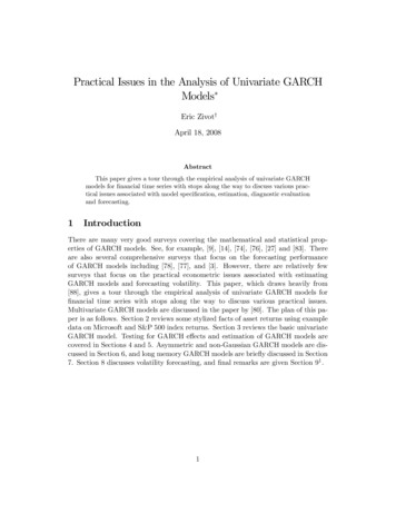
we found that the surface was fairly at around the optimal solution, and estimates of theparameters could uctuate widely, without signi cant improvement in the SSE. By assumingthe market price of risk, , to be zero, lead to very little change in the objective function. As aresult, in what follows, we report the results when our optimizations were conducted over the 5remaining values.Table 1a reports the parameter estimates for the HN Model for each of the 10 six monthperiods, from January 1991 to the last 6 month period in 1995. Table 1b shows the same resultsfor the NGARCH model. For both models we report the estimates of the 4 parameters, namely 0 , 1 , 2 and !, as well as the implied estimate of the initial local volatility, h0 . Our results forthe HN model are generally in the same range as those established by HN. For example, theirparameter estimates were b0 5:02E ¡ 06, b1 0:58, b2 1E ¡ 06 ! 421, and the marketprice of risk, was not signi cant.Insert Tables 1a and 1b HereThe tables also report the stationary volatility, and the nal local volatility that exists at theend of the period. The long run stationary volatility estimates produced by both the NGARCHmodel and the HN model appear to be very stable, not deviating too far from about 17% peryear. Figure 1 shows the time series of these \local" volatilities for each year. The parametersfor the process are estimated using the rst six months of data, and then these values are usedwith the actual daily time series of the index to generate the local volatilities over the entireyear. The time series produced by these two models over each of the 5 years are shown in the rst two panels of Figure 1. In most years the time series of local volatility in the NGARCHmodel appears to be less volatile than in the HN model. The third panel in Figure 1 shows thetime series of implied volatilities obtained by minimizing the sum of squared errors in optionprices using the Black Scholes model for each of the 52 weeks in the year. This time series isthe least volatile.Insert Figure 1 HereSince our primary goal is to investigate the performance of our two GARCH models in pricingoptions, we now turn attention to examining the residuals associated with our models.In what follows we de ne moneyness as M (St ¡ X) St , where X is the strike price.Deep-out-the money options are de ned as M ¡0:04; out-the-money contracts are de ned as¡0:01 M · 0:04; at-the-money contracts have ¡0:01 M · 0:01; in the money contractshave 0:01 M · 0:04, and deep in the money contracts have M 0:04. Expiration datesare bucketed into 3 groups: near term contracts have maturities between 10 and 45 days; midterm contracts have maturities between 46 and 90 days; and long term contracts have maturities8

between 91 and 200 days. Residuals are computed as theoretical prices less actual prices. Unlessstated otherwise, all contract prices have been normalized so that the underlying asset price is 1:0.All the residuals over the in-sample periods are rst analyzed to assess whether the models aremisspeci ed. Figure 2 shows box and whisker plots for residuals generated by the three modelscategorized by moneyness and maturity. If there were no systematic biases in the models, theresiduals should be centered around zero, for each moneyness-maturity category.Insert Figure 2 HereThe plots reveal large volatility skew and smile patterns associated with the Black Scholesmodel. The biases for this model are particularly large on average. In particular, on average,deep in-the-money contracts are priced too low and deep out-the-money contracts are pricedtoo high with the bias increasing, in raw dollar terms, with maturity. That is, on average,at-the-money and out-the-money Black Scholes option prices are higher than actual prices whiledeep in-the-money contracts are priced too low.The box and whisker plots clearly reveal that the two GARCH models remove a signi cantfraction of the strike price bias, for each maturity bucket. There are still patterns, on average inthe Heston-Nandi model. Speci cally, away from the money contracts are priced too low, whileat-the money contracts are priced a bit too high. The NGARCH model appears to remove moreof the strike price bias. Moreover the interquartile range of residuals appears to be tighter asdoes the 95% con dence intervals.By normalizing the index price to be 1:0 over the entire ve years, the option price residualshave a very natural interpretation. An error of 0:01 for example, can be viewed as a error ofone cent, or 1% of the underlying. However, perhaps a better criterion to assess the t of themodels is to examine the percentage error in pricing. Since out-the-money options have smallactual prices, this criterion magni es the ability of di erent models in explaining the prices ofout-the-money contracts.Figure 3 shows the plots of these percentage errors. Since the percentage errors of deepin-the money contracts are so small relative to the other 4 moneyness buckets, the gure onlyshows the pattern over the remaining 4 categories.Insert Figure 3 HereThe results are very revealing. First, note the huge biases in Black Scholes prices. Fordeep in, in, and at-the-money contracts, the interquartile range of theoretical prices is within3 percentage points of actual prices. However, the bias in percentage errors increases as the9

contract moves out of the money. For example, on average, deep out-the-money options aremispriced by almost 50%. More than one in four contracts in this category were mispriced byat least 100%, and the 95% con dence interval extended to 200%. As Figure 3 illustrates, thebias holds true for all maturity buckets.The two GARCH models perform much better, with the NGARCH model doing fairly well,even for the deep-out-the money contracts. For example, this model shows almost no moneynessbias for each of the three maturity buckets. Of course the interquartile range expands as wemove out of the money, but this is to be expected, since the denominator is getting smaller.The HN model produces intermediate results. Our results here con rm other studies, such asthose by Duan (1995) and Heston and Nandi (2000) that have shown that GARCH models arecapable of explaining a signi cant portion of the volatility strike price bias.We now investigate the out-of-sample performance on the models using models that wereestimated over the rst six months, and residuals generated from the last 6 months of each year.The pattern of these residuals in the out of sample period are similar to the in sample period forthe rst six months. For example, Figure 4 compares the out-of-sample box and whisker plotsof the two GARCH models.Insert Figure 4 HereIn comparing the residuals of the NGARCH and HN models, their magnitudes appear tobe of the same order, although for out-the-money options there does appear to be more bias inthe HN model. To establish which of the two GARCH models is better, we compare the outof-sample predictions, contract by contract. We compute the absolute error for each contractproduced by each model, and compute the di erence between the two values. Figure 5 provideshistograms of these di erences by maturity and moneyness. Negative values indicate that theNGARCH model produced more precise values.Insert Figure 5 HereTable 2 summarizes the proportion of contracts for which the HN model outperformed theNGARCH model in the out of sample periods. For almost all categories the NGARCH modelproduces smaller residuals than the HN model. The most dramatic di erences occur in the deepout the money contracts. For these contracts the HN model is unable to explain the volatilitystrike bias and systematically underperforms.Insert Table 2 HereWe next investigate how the out of sample errors behave as the time since calibration increases. Speci cally, it seems plausible that the conditional forecasts of option prices one week10

after the parameters are estimated might be relatively small compared to conditional optionprices generated several months after the parameters are estimated. To address this issue we rst grouped all the residuals produced by a model into moneyness and maturity buckets andthen looked at the distribution of the percentage pricing errors as the time since estimationincreased, from one week through 25 weeks. Figure 6 compares the distribution of residuals for6 di erent out-of-sample periods. In particular, a box and whisker plot is provided for eachmonth, from the rst out of sample month to the last.Figure 6a shows the result

Scholes model of Dumas, Fleming and Whaley (1998) that uses a separate implied volatility for each option to t the volatility \smile". In contrast, previous empirical tests, conducted by Dumas et. al., showed that the implied binomial tree-deterministic volatility models were out-performed by the ad hoc Black Scholes model.