Transcription
Prediction Models for Dynamic Demand ResponseRequirements, Challenges, and InsightsSaima Aman* , Marc Frincu† , Charalampos Chelmis† , Muhammad Noor† , Yogesh Simmhan‡ , Viktor K. Prasanna†*Computer Science Department, University of Southern California, Los Angeles, CAElectrical Engineering Department, University of Southern California, Los Angeles, CA‡Supercomputer Education and Research Centre, Indian Institute of Science, Bangalore, IndiaEmail: saman@usc.edu, frincu@usc.edu, chelmis@usc.edu, mnoor@usc.edu, simmhan@serc.iisc.in, prasanna@usc.edu†Abstract— As Smart Grids move closer to dynamic curtailmentprograms, Demand Response (DR) events will become necessarynot only on fixed time intervals and weekdays predeterminedby static policies, but also during changing decision periodsand weekends to react to real-time demand signals. Uniquechallenges arise in this context vis-a-vis demand prediction andcurtailment estimation and the transformation of such tasksinto an automated, efficient dynamic demand response (D2 R)process. While existing work has concentrated on increasingthe accuracy of prediction models for DR, there is a lack ofstudies for prediction models for D2 R, which we address in thispaper. Our first contribution is the formal definition of D2 R, andthe description of its challenges and requirements. Our secondcontribution is a feasibility analysis of very-short-term predictionof electricity consumption for D2 R over a diverse, large-scaledataset that includes both small residential customers and largebuildings. Our third, and major contribution is a set of insightsinto the predictability of electricity consumption in the context ofD2 R. Specifically, we focus on prediction models that can operateat a very small data granularity (here 15-min intervals), forboth weekdays and weekends - all conditions that characterizescenarios for D2 R. We find that short-term time series and simpleaveraging models used by Independent Service Operators andutilities achieve superior prediction accuracy. We also observethat workdays are more predictable than weekends and holiday.Also, smaller customers have large variation in consumption andare less predictable than larger buildings. Key implications of ourfindings are that better models are required for small customersand for non-workdays, both of which are critical for D2 R. Also,prediction models require just few days’ worth of data indicatingthat small amounts of historical training data can be used tomake reliable predictions, simplifying the complexity of big datachallenge associated with D2 R.I. I NTRODUCTIONElectricity consumption optimization is critical to enhanceelectric grid reliability and to avoid supply-demand mismatches. Utilities have long used demand response (DR) forachieving customer-driven curtailment during peak demandperiods to maintain reliability [1]. Traditionally, planning andnotification for DR is done a day ahead of the day whencurtailment is to be performed [2]. However, the Smart Gridis transitioning towards dynamic demand response [3], inwhich the utility provider needs to perform DR at a fewhours’ advance notice whenever necessitated by dynamicallychanging conditions of the grid. We formally define DynamicDemand Response as follows:TABLE I: Comparison of DR and D2 R characteristics andchallengesGoalHorizonData/control granularityData rateDRadvance planningday aheadcoarsemonthly billingTiming and durationfixed and pre-definedExtent of curtailmentfixedCustomer selectionChallengesselected a-priorilabor intensive, dataunavailability, inability to adaptD2 Rdynamic adaptationhours aheadfinereal-time data fromsmart metersflexible, dynamicallydetermineddynamically determined/adjustabledynamically lexity,datadelugeDefinition 1: Dynamic Demand Response (D2 R) is theprocess of balancing supply and demand in real-time andadapting to dynamically changing conditions by automatingand transforming the demand response planning process.Several factors drive the transition towards D2 R; mostnotable the integration of renewable energy sources, which dueto their intermittent, non-dispatchable, and uncertain natureresult in supply instability [2]. The need to curtail at timeperiods which were traditionally considered non-peak periods,such as weekends, as a result of such instabilities is beyondexisting DR policies. The need to curtail any time as a resultof such instabilities is beyond existing DR policies, which aretraditionally defined for workdays, and usually in hot summerafternoons [4], [1]. Besides, Plug-in electric vehicles (PEVs)can introduce spikes in consumption at arbitrary times duringthe course of a day [5], whereas special events can result inincreased load on weekends. The key differences between DRand D2 R are summarized in Table I.In DR, the focus has been on large industrial and commercial customers [2], selected a-priori, who are expected tocontribute large-sized curtailment. With increasing adoptionof smart meters [6], [3], and home energy management andautomation systems [7], [2] however, the participation of smallcustomers in demand side management is increasing. Theelectricity demand of such small customers might be easier toregulate (i.e. shift or shave) as compared to the load of com-
mercial entities, however, consumption prediction for smallcustomers and at high temporal granularity is challenging [8],[9]. One of the key implications of involving small customerswould be to dynamically and optimally select customers forparticipation in curtailment [2] and request only the minimumcurtailment required to avoid fatigue and loss of interest in thecustomers [1].While existing work has focused on improving consumptionprediction models[1], [9], to date, there has been little studyon the differences in consumption characteristics of variouscustomer types and their impact on prediction models’ accuracy. Existing studies have shown that consumption predictionaccuracy is high when consumption values of individualcustomers are aggregated together [6], [10], [11]. This isattributed to the law of large numbers such that larger thenumber of customers in an aggregated group, the lower theprediction error for the group [12]. Predictions for aggregatedgroups make it impossible to discover curtailment potential ofindividual customers, which is necessary for wider adoption ofD2 R. Models that work well for large commercial customerswith smaller consumption variability over time, could be lessefficient for small residential customers, whose consumptionpattern fluctuates significantly. Thus, it is necessary to identifyeffective methods for predicting demand for diverse customers.In this paper, we compare six short-term electricity consumption prediction models. Our study differs from previouswork and focus specially to D2 R challenges, in that: it deals with small, highly variable, individual customerconsumption, as well as relatively larger and more stablebuilding consumption; consumption data granularity is very small (i.e., 15min interval) for appropriately timing the requests fordynamic demand response (D2 R) [1], as opposed to priorwork on hourly or higher granularity predictions; it focuses on short-term predictions (hours ahead) required for (D2 R) [1], as opposed to most prior work onday-ahead predictions; it evaluates the relationship between prediction accuracyand day type, i.e., workday versus weekends or holidays.These distinctions make the insights we draw greatly usefulfor researchers and practitioners in the smart grid domain.Our goal is to get a comprehensive understanding of theperformance of prediction models for D2 R. Prediction modelsused for D2 R should balance conflicting requirements of highprediction accuracy, low compute time for training andprediction, and reliability at any time of the week and fordiverse customers. This paper can be considered as firstattempt in studying prediction models specifically from thisperspective.II. P REDICTION M ODELS FOR D 2 ROur work advances previous research on analyzing performance of prediction models, such as [8], [2], [13], but differsfrom them in experiments and analysis focused specificallyon D2 R. Electricity consumption prediction models can bebroadly categorized into three groups [14]: 1) simple averagingmodels; 2) statistical models like regression and time seriesmodels; and 3) artificial intelligence and machine learningmodels (AI/ML) like neural networks and support vector machines [14] [10], [15], [8]. As many AI/ML methods involvelonger training times, they may not be suitable for near realtime predictions required for D2 R, and hence not consideredhere.In the following, we describe the models considered inour study. While the models used in our analysis are notexhaustive, they represent the most commonly used algorithmsin demand-response systems [1], [8] and meet the requirementsfor D2 R predictions as mentioned previously.A. Averaging ModelsAveraging models are popular among utilities and ISOs[16][17][18] due to their simplicity [19]. Averaging modelsmake predictions based on linear combinations of consumptionvalues from limited historical data. Averaging models havebeen shown to perform as well as advanced machine learningand time-series models [8] while considerably reducing thecomputational need for large-scale predictive analysis of homeenergy data. In our study, we consider three popular averagingmodels and a Time of Week (ToW) model, as described below:1) New York ISO Model (NYISO): It predicts for the nextday by taking hourly averages of the five days with highestaverage consumption value among a pool of ten previous days,starting from two days prior to prediction [16]. It excludesdata from weekends, holidays, past DR event days or dayswith sharp drop in the energy consumption.2) California ISO Model (CAISO): It predicts for the nextday by taking hourly averages of the three days with highestaverage consumption value among a pool of ten previous days,excluding weekends, holidays, and past DR event days [17].3) Southern California Edison Model (CASCE): It predictsfor the next day by taking hourly averages across past tenimmediate or similar days, excluding weekends, holidays, andpast DR event days [19], [18].4) Time of Week Average Model (ToW) : It predicts for each15-min interval in a week by taking average over all weeks inthe training dataset. It captures consumption variations overthe duration of a day , i.e., from day to night, and acrossdifferent days of the week. Time related features are importantfor electricity consumption [20] as it is closely tied to humanschedules and activities.B. Regression ModelsRegression models combine several independent featuresto form a linear function. Commonly used regression models for electricity consumption prediction are regression treemodels [21], probabilistic linear regression, and gaussian process regression models [22]. Hybrid methods that combineregression-based models with other models have also beenused for short term load prediction [23]. A multiple linearregression model for load prediction was presented in [26].A non-linear and non-parametric regression model for nextday half-hourly load prediction was employed in [27] for
stochastic planning and operations decision making. In otherstudies, Support Vector Machines have also been used for loadforecasting [24], [25].We use regression trees [28] in this study. A regressiontree recursively partitions data into smaller regions until eachregion can be represented by a constant or a linear regressionmodel. Its key advantage is its flowchart or tree representationthat enables domain users to interpret the impact of differentfeatures on predicted values [21]: Also, once trained, predictions are fast to compute by a tree look-up [1].C. Time Series ModelsTABLE II: Description of microgrid and utility datasets.Number of participantsData collection periodData pointsClient typeMean consumption (kWh)Average variance (kWh)Campus Microgrid1704 years4 years 365 days 96 intervals 140 103points per building 16 106 pointstotalbuildingslarge (30.52 7.65)122.56Utility Dataset893 months3months 30days 96 intervals 8.5 103points per customer 0.73 106points totalhouseholdssmall (0.22 0.15)0.026A Time Series model predicts future values based on recentobservations. One of the early reviews for time series basedmodels for load forecasting is given in [29]. A comparison oftime series methods for load forecasting with other methods ispresented in [30]. A time series method for short to mediumterm load forecasting (few hours to few weeks ahead) of hourlyloads was proposed in [31].In this study, we use Auto-Regressive Integrated MovingAverage (ARIMA) [29]. ARIMA is defined in terms of threeparameters: d, the number of times a time series needs tobe differenced to make it stationary; p, the auto-regressiveorder, that denotes the number of past observations includedin the model; and q, the moving average order that denotes thenumber of past white noise error terms included in the model.These parameters are derived from the Box-Jenkins test [32].III. E XPERIMENTAL S ETUPA. Dataset DescriptionElectricity consumption data: Our data for small customersis drawn from a major California power utility. It comprises of15-min kWh values from 89 household customers, collectedbetween Feb 2013 and Apr 2013. The data1 for the buildinglevel large customers comes from USC campus microgrid [33],[3]. It comprises of 15-min kWh values from 170 USC campusbuildings, collected between Jul 2009 and Jun 2013 [33], [3]. Itrepresents large customers of diverse type: teaching and officespaces, residential, and administrative buildings. For bothdatasets, we excluded customers with major discontinuitiesin data, and used linear interpolation for minor gaps. Keyproperties of the datasets are summarized in Table II, andtheir distribution is shown in Figure 1. For more details onthe datasets, the readers are referred to [34].Weather data: We obtained curated weather data fromNOAA [35], [36] We used hourly temperature observations,which were interpolated to 15-min values.Schedule Data: It was obtained for the campus dataset comprised of information on working days, holidays, and semesterdurations (for campus dataset). We used this information tocompare the performance of workday versus non-workdayperformance of the models.1 Availablefrom the USC Facility Management Services (FMS).Fig. 1: Probability density function (PDF) of average kWhconsumption per 15-min interval of campus buildings. Embedded: the PDF of utility area customers.B. Prediction Models’ ConfigurationFor the averaging models and regression tree models, wespilt both datasets in 2:1 where 2 parts were used for trainingand 1 part for testing. For both datasets, we build one prediction model per customer. For the regression tree models, weselected the feature combination that offered the best prediction accuracy based on our previous work [21]: day of week,semester, temperature, and holiday/working day flag. The timeseries models are trained using a sliding window of 8 weekspreceding the prediction period to predict for three horizons:1, 4, and 24 hours. For the time series ARIMA model, theparameters were found to be (8, 1, 8) for the campus datasetand (4, 1, 4) for the utility dataset.The prediction models’accuracy was compared using the Mean Absolute PercentageError (MAPE) [1].IV. P ERFORMANCE A NALYSISObservation 1: Prediction accuracy is higher for customerswith high consumption. We compare how accuracy varieswith customer size, which is defined in terms of the average consumption value in a 15-min interval. Due to space
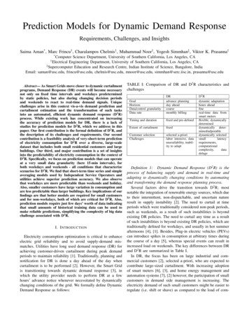
TABLE III: Average MAPE (with standard deviation) for TS1hr for groups of buildings/customers.UtilityCampusavg. kWhkWh 5kWh 55 kWh 1515 kWh 50kWh 50workdays0.3075 0.13090.1204 0.06490.0743 0.03820.0610 0.03080.0392 0.0147all days0.3054 0.12690.1186 0.06230.0750 0.03550.0617 0.02930.0416 0.0199Fig. 2: TS-1hr MAPE as a function of average kWh.limitations we report here results for the Time Series (1hr) model in Fig 2. Results for the rest of the models areavailable at [34]. Higher errors for small sized customers canbe observed in both datasets. TS-1hr, the best performingmethod achieves 30.74% average MAPE (Figure 3c), whereas,CASCE, the best performing averaging method, is far worse,with average MAPE 45.91% for utility customers. We furtherquantify the relationship of customer size and prediction errorby dividing campus buildings in four groups according toaverage consumption and calculating average MAPE for eachgroup. Table III summarizes the results. Evidently, the averageMAPE drops significantly with consumption from 12.04%for smaller buildings to 3.92% for large consumers. Thisresult corroborates previous observations of higher accuracyfor larger aggregated consumption prediction [6], [10], [11].The discrepancy in prediction accuracy between small andlarge customers can be explained by two factors. First, thereis higher variability in small customers [34], i.e., households,where even switching on or off a light bulb can cause a noticeable change in consumption. Second, activities in campusbuildings are expected to be periodic, governed by pre-definedschedules and hence expected to be less variable. However, forsmaller customers, even a small offset in the predicted kWhvalue results in a higher percentage error value as a result ofthe difference between predicted and actual value being highproportionally to large customers.Insight 1: D2 R requires higher accuracy models for smallcustomers.Observation 2: Few recent observations are better predictors than large sets of historical observations. Averagingmodels perform well while using only a small set of recenthistorical data (i.e., 2-3 weeks). We found CASCE (Figure3) to be particularly effective for workdays, while ARIMAachieves the best performance while only requiring few training data. According to Figure 3, even simple heuristics such asthe Time of Week model perform reasonably well with morerecent data (i.e., ToW performs better when trained on dataspanning 2 months than when using data covering a periodof 2 years). We conclude that historical data of extendedtime spans enclose consumption patterns that change overtime introducing “noise” and deteriorating prediction accuracy.Other researchers have also found that increasing the trainingdata did not improve accuracy [8].Insight 2: Prediction models for D2 R relying on few datacan maintain high short-term prediction accuracy while significantly reducing storage requirements and computationalcomplexity associated with training and latency (i.e., predictions can be made in real-time). It also implies that reliablepredictions for new buildings or customers can be initiatedsooner without waiting to accumulate large training data.Observation 3: Simple averaging models are inadequatefor DR during weekends. In our experiments, we evaluatedmodels’ performance with respect to all days versus justworkdays (Figure 3b). For workdays, the three ISO/utilitymodels achieve lower than 20% MAPE for over 80% ofthe campus buildings. CASCE is the best among them, withan average MAPE of 10.93%. However, when including alldays, CASCE’s performance is affected the most. Its averageMAPE increases from 10.93% to 17.29%, indicated by a shiftof the CDF line to the right in Figure 3d. For experimentsinvolving weekends, we used a modified version of CASCE,which was trained on all days of the week. The degradationin CASCE’s performance when including weekends can beattributed to weekend loads being different than weekdaysfor both campus buildings and utility datasets due to different schedules. Contrary, ARIMA’s accuracy deteriorates onlyslightly for weekends. For TS 1-hour model, MAPE increasesby 1.13% (from 7.05% to 7.13%). Time series model benefitsfrom temporal locality and thus does not distinguish betweenworkdays and weekends. The regression tree and time ofweek models are unaffected as both models inherently capturethe workday/weekend information. Specifically, our regressiontree model uses day of week and workday/holidays as features,whereas time of week prediction is done by taking averagesindividually for each day of the week.Insight 3: D2 R requires the development of accurate modelsfor all days of the week. Traditional DR involved industrialcustomers [2] with weekends considered as non-peak. InsteadD2 R can be initiated at any time involving both industrial andresidential customers.Observation 4: ARIMA achieves the best predictionaccuracy for very-short-term predictions. For both datasets,the time series 1-hour model achieves the best performance.It’s accuracy however deteriorates for longer horizons. While
(a) Campus dataset – Workdays(c) Utility dataset – Workdays(b) Campus dataset – All days(d) Utility dataset – All daysFig. 3: CDF of MAPE values for campus and utility datasets.this result is well known [1], the confirmation in the contextof near-real-time consumption prediction makes it a goodcandidate for D2 R. For campus buildings, average MAPEincreases from 7.05 4.4% to 13.05% for 4-hour horizon, anddown to 26.38% for 24-hour horizon for workdays (Figure 3a).For utility customers, TS 1-hour outperforms other predictiontechniques for workdays, achieving MAPE below 30% for80% of the customers (Figure 3c). Combining autoregressionwith moving averaging, ARIMA can approximate temporallocality in electricity consumption. However, as the predictionhorizon increases so does the volatility in the consumptiontime series data. Therefore, continuous re-training of ARIMAmodels is necessary for high accuracy to be maintained.Insight 4: While TS 1-hour provides best results, its highertraining cost [1] makes it problematic for D2 R.Observation 5: Models that try to capture global patterns over long time periods are not suitable for D2 R.We found both the regression tree and Time of the Weekmodels to be ineffective for D2 R, even though we havedemonstrated their usefulness for medium and long-term predictions previously [21], [1]. Also, the results indicate thatusing additional features, as in regression tree model, did notimprove prediction performance.Insight 5: Regression tree model is not suited for short termprediction required in D2 R, though it has been found usefulfor medium and long-term predictions [21], [1].V. C ONCLUSIONSWe described how dynamic demand response (D2 R) requires very-short-term consumption prediction to make realtime adaptive decisions about curtailment. Prediction modelsused for D2 R should balance conflicting requirements of highprediction accuracy, low compute time for training and prediction, and reliability at any time of the week and for diversecustomers. We analyzed six prediction models leading to keyinsights relevant for D2 R. 1) Our results indicate that thereis an inherent randomness associated with small customers,which makes it harder to reliably predict their energy con-
sumption compared to larger customers. Thus, D2 R requireshigher accuracy models for small customers. 2) Predictionmodels for D2 R relying on few data can maintain high shortterm prediction accuracy while significantly reducing storagerequirements and computational complexity associated withtraining and latency. 3) D2 R requires the development ofaccurate models for all days of the week. 4) While Time Series1-hour provides best results, its higher training cost makes itproblematic for D2 R. 5) Regression tree model is not suitedfor short term prediction required in D2 R, though it has beenfound useful for medium and long-term predictions. For futureenergy management systems, researchers need to design bettermodels, personalized for individual customers that leveragebig data available in D2 R environments to overcome inherentrandomness in consumption profiles of individual customers.ACKNOWLEDGMENTThis material is based upon work supported by the UnitedStates Department of Energy under Award Number numberDE-OE0000192, and the Los Angeles Department of Waterand Power (LA DWP). The views and opinions of authorsexpressed herein do not necessarily state or reflect those ofthe United States Government or any agency thereof, the LADWP, nor any of their employees.R EFERENCES[1] S. Aman, Y. Simmhan, and V. K. Prasanna, “Holistic measures forevaluating prediction models in smart grids,” IEEE Transactions onKnowledge and Data Engineering (to appear), 2014.[2] H. Ziekow, C. Goebel, J. Struker, and H.-A. Jacobsen, “The potentialof smart home sensors in forecasting household electricity demand,” inIEEE International Conference on Smart Grid Communications, 2013.[3] Y. Simmhan, S. Aman, A. Kumbhare, R. Liu, S. Stevens, Q. Zhou, andV. Prasanna, “Cloud-based software platform for data-driven smart gridmanagement,” IEEE/AIP Computing in Science and Engineering, 2013.[4] S. Park, S. Ryu, Y. Choi, and H. Kim, “A framework for baselineload estimation in demand response: Data mining approach,” in IEEEInternational Conference on Smart Grid Communications, 2014.[5] K. Clement-Nyns, E. Haesen, and J. Driesen, “The impact of chargingplug-in hybrid electric vehicles on a residential distribution grid,” IEEETransactions on Power Systems, vol. 25, no. 1, 2010.[6] Y. Simmhan and M. Noor, “Scalable prediction of energy consumptionusing incremental time series clustering,” in Workshop on Big Data andSmarter Cities, 2013 IEEE International Conference on Big Data, 2013.[7] S. Aman, Y. Simmhan, and V. Prasanna, “Energy Management Systems: State of the Art and Emerging Trends,” IEEE CommunicationsMagazine, Ultimate Technologies and Advances for Future Smart Grid(UTASG), 2013.[8] D. Lachut, N. Banerjee, and S. Rollins, “Predictability of energy use inhomes,” in International Green Computing Conference, 2014.[9] H. Y. Noh and R. Rajagopal, “Data-driven forecasting algorithmsfor building energy consumption,” in SPIE 8692, Sensors and SmartStructures Technologies for Civil, Mechanical, and Aerospace Systems,2013.[10] F. Martinez-Alvarez, A. Troncoso, J. Riquelme, and J. A. Ruiz, “Energytime series forecasting based on pattern sequence similarity,” IEEETransactions on Knowledge and Data Engineering, vol. 23, no. 8, 2011.[11] W. Shen, V. Babushkin, Z. Aung, and W. L. Woon, “An ensemblemodel for day-ahead electricity demand time series forecasting,” inInternational Conference on Future Energy Systems (ACM e-Energy),2013.[12] T. Hossa, A. Filipowska, and K. Fabisz, “The comparison of mediumterm energy demand forecasting methods for the need of microgridmanagement,” in IEEE International Conference on Smart Grid Communications, 2014.[13] A. Veit, C. Goebel, R. Tidke, C. Doblander, and H.-A. Jacobsen,“Household electricity demand forecasting - benchmarking state-of-theart methods,” in ACM e-Energy Conference, 2014.[14] H. K. Alfares and M. Nazeeruddin, “Electric load forecasting: Literaturesurvey and classification of methods,” International Journal of SystemsScience, vol. 33, no. 1, 2002.[15] S. D. Ramchurn, P. Vytelingum, A. Rogers, and N. R. Jennings, “Puttingthe ’Smarts’ Into the Smart Grid: A Grand Challenge for ArtificialIntelligence,” Communications of the ACM, vol. 55, no. 4, 2012.[16] “Emergency Demand Response Program Manual, Sec 5.2: Calculationof Customer Baseline Load (CBL),” New York Independent SystemOperator (NYISO), Tech. Rep., 2010.[17] “CAISO Demand Response User Guide, Guide to Participation inMRTU Release 1, Version 3.0,” California Independent System Operator(CAISO), Tech. Rep., 2007.[18] “10-Day Average Baseline and Day-Of Adjustment,” Southern California Edison, Tech. Rep., 2011.[19] K. Coughlin, M. A. Piette, C. Goldman, and S. Kiliccote, “Estimatingdemand response load impacts: Evaluation of baseline load models fornon-residential buildings in California,” Lawrence Berkeley NationalLab, Tech. Rep. LBNL-63728, 2008.[20] E. A. Feinberg and D. Genethliou, “Load forecasting,” Applied Mathematics for Restructured Electric Power Systems: Optimization, Control,and Computational Intelligence, pp. 269–285, 2005.[21] S. Aman, Y. Simmhan, and V. K. Prasanna, “Improving energy useforecast for campus micro-grids using indirect indicators,” in IEEEWorkshop on Domain Driven Data Mining, 2011.[22] J. Z. Kolter and J. F. Jr, “A large-scale study on predicting andcontextualizing building energy usage,” in AAAI Conference on ArtificialIntelligence, 2011.[23] H. Mori and A. Takahashi, “Hybrid intelligent method of relevantvector machine and regression tree for probabilistic load forecasting,”in IEEE International Conference and Exhibition on Innovative SmartGrid Technologies (ISGT Europe), 2011.[24] B.-J. Chen, M.-W. Chang, and C.-J. Lin, “Load forecasting usingSupport Vector Machines: a study on EUNITE competition 2001,” IEEETransactions on Power Systems, vol. 19, no. 4, pp. 1821–1830, 2004.[25] Z. Aung, M. Toukhy, J. Williams, A. Sanchez, and S. Herrero, “Towards accurate electricity load forecasting in smart grids,” in DBKDA2012, The Fourth International Conference on Advances in Databases,Knowledge, and Data Applications, 2012, pp. 51–57.[26] T. Hong, M. Gui, M. Baran, and H. Willis, “Modeling and forecastinghourly electric load by multiple linear regression with interactions,” inPower and Energy Society General Meeting, 2010 IEEE, 2010, pp. 1–8.[27] S. Fan and R. Hyndman, “Short-term load forecasting based on asemi-parametric additive model,” IEEE Transactions on Power Systems,vol. 27, no. 1, 2012.[28] L. Breiman, J. H. Friedman, R. A. Olshen, and C. J. Stone, Classificationand Regression Trees. Chapman and Hall, 1984.[29] M. Hagan and S. M. Behr, “The time series approach to short term loadforecasting,” IEEE Transactions on Power Systems, vol. 2, no. 3, 1987.[30] J. W. Taylor, L. M. de Menezes, and P. E. McSharry, “A comparisonof univariate methods for forecasting electricity demand up to
Email: saman@usc.edu, frincu@usc.edu, chelmis@usc.edu, mnoor@usc.edu, simmhan@serc.iisc.in, prasanna@usc.edu Abstract— As Smart Grids move closer to dynamic curtailment . and day type, i.e., workday versus weekends or holidays. These distinctions make the insights we draw greatly useful for researchers and practitioners in the smart grid .