Transcription
Surface Runoff: A Rainfall Simulator ForWash-Off Modelling And Road SafetyAuditing Under Different RainfallIntensitiesSimone A.Professor – University of Bologna – DISTART StradeVignali V.Ph.D Student – University of Bologna – DISTART StradeBragalli C.Researcher – University of Bologna – DISTART Costruzioni IdraulicheMaglionico M.Researcher – University of Bologna – DISTART Costruzioni IdraulicheSYNOPSISThe great traffic and vehicle average speed increase in recent years have improved road pavementsperformance standards. Road surface must be designed, built and maintained to offer the highest activesafety to drivers. This is very important during rainfall events, because the water collected on roadpavements produces a drastic decrease of skid resistance and visual distance. So water film depthestimation is one of the most important factor on road safety.Moreover during rainfall events the rainfall wash pollutants collected on road pavements and dissolve themin urban drainage with an important environmental impact.In this paper has been studied and modelled the pollutants wash-off on road pavements and the vehicle-roadinteraction in terms of water film depth. The laboratory equipment consists of an artificial rain system,capable of simulating variable rainfall intensities by different nozzles and by a controlled water dischargesystem to collect the water flowing from the road surface.To reproduce different rainfall intensities, three nozzles were used and calibrated according to rainfallintensity, drop dimension distribution and medium drop diameter.From rated flow calculation it has been investigated: the effect of different rainfall intensity regimes on pollutants wash-off and safety; the effect of different surface slope on wash-off and safety; the effect of water film depth on skid resistance and safety.The data collected in this way have been submitted to an in-depth analysis, which has provided particularlyinteresting and significant results regarding design and maintenance of roads according to security andenvironmental standards.
Surface Runoff: A Rainfall Simulator ForWash-Off Modelling And Road SafetyAuditing Under Different RainfallIntensitiesINTRODUCTIONThe rainfall events on an asphalt surface produce two different effects: the first on the water film, andconsequently on road safety, and the other on the road waste runoff, which is directly connected to theenvironmental impact. In this paper has been studied and modelled the pollutants wash-off on roadpavements and the vehicle-road interaction in terms of water film depth.An understanding of pollutant wash-off characteristics is essential to estimate and to minimise the impacts ofpollutants on the environment. Stormwater quality models typically view stormwater pollution as a two stageprocess, pollutant build-up and pollutant wash-off. Build-up is the accumulation of pollutants on thecatchment surface during dry periods and wash-off is the removal of the pollutants by rainfall and runoff(Vaze and Chiew, 2002). The few studies on pollutant build-up, since the detailed experimental pollutantaccumulation studies of Sartor and Boyd in 1972, agree that surface pollutant load increase duringantecedent dry weather period, but there are doubts on the assumption that the buildup starts from zero aftera rain event is realistic. Depending on the rainfall and runoff characteristics, part of the available pollutant isremoved from the surface as wash-off, the remainder becomes a part of the fixed load as it attaches itself tothe surface. During drying, part of the free load of the build-up process can attach itself to the surfacecontributing to the fixed load amount. The experimental study on an urban road surface in Melbourne (Vazeand Chiew, 2002) has shown that common storms only remove a small proportion of the total surfacepollutant load, also it has suggested that the rainfall and runoff disintegrate and dissolve more surfacepollutant that they can actually remove.The road surface conditions and temperature are very important for the adherence values. In real conditionsthe road could be contaminated with dust, mud or sand, or covered with water, ice or snow. On the wetroads, when the water thickness is very low and motor vehicle speed in normal range, it could be observed asomewhat decrease of adherence. This fact could be explain due to the diminish value of adhesion frictionon lubricated surfaces. The peak and slide values of the longitudinal force coefficient on wet road comparedto the values on dry road are presented in figure 1.Figure 1: Comparison between dry and wet road adherence conditions [Pauwelussen, 2002]
In addition, the influences of load and vehicles speed are depicted in figure 2.Figure 2: Comparison of load and speed effect on dry and wet roads (radial truck tyre) [Pauwelussen,2002]When the water layer thickness and vehicle speed increase the hydroplaning phenomenon appear. So, thetyre is lifting from the road surface due to the pressure created by water under tyre. The magnitude ofhydroplaning depends on: water conditions (water depth, surface texture and drainage); pressure distribution in contact area; tyre patterns design (groove capacity on removing water).The tyre behaviour between the state in which hydroplaning begin and the full (total) hydroplaning state, iscommonly described with the "three-zone concept" (Giannini and Noli, 1974). As can be seen in figure 3,zone A (unbroken water film) is in forward region of the contact area where the hydrodynamic pressure liftsand completely separates the tread from the road. In this region the water film remains unbroken and thelocal coefficient of friction is substantially zero. Zone B (transition zone) is the region where a progressivebreakdown of the water is dissipated but where a thin film layer of water still remains. In this region theeffective coefficient of friction varies widely. Zone C ("dry" contact) is the region where the lubrication film hasbeen substantially removed and the road frictional forces can be generated. The image of contact area of aheavy truck tyre that rolls on a smooth glass surface covered with water is shown in figure 4. The keyobjective in order to improve the adherence in this case is to increase the length of zone C through anoptimum tread pattern design.Figure 3: The three-zone concept of contact area [Giannini and Noli, 1974]
Figure 4: Contact area of a truck tyre rolling through a film of water [Pauwelussen, 2002]To analyse the pollutant wash-off on road surface and the vehicle-road interaction in term of water filmdepth, a rainfall simulator has been developed. The rainfall simulation is a very useful method to study therain water distribution and its effects on a catchment area, as waterproof surfaces (Lorenzini and Becchi,2000), road pavements (Domenichini and La Torre, 1997), road transitional areas between planimetriccurves (Domenichini and Remedia, 1992), soil erosion (Romkens et al, 2001), etc. In this way it’s possible totake a lot of measures without waiting for the natural rain and to work with a constant rain intensity withoutthe natural rain intensity variability. So it has been developed the device described in this paper, to aim ofunderstanding the bituminous surfaces runoff and the pollutants wash-off phenomenon.RAINFALL SIMULATORThe experimental device is composed from a rainfall simulator, a structure with adjustable inclination onwhich is placed a bituminous surface, a system to remove external rainfall to the bituminous surface and acollection system of internal rainfall to bituminous surface, set at the final section (figures 5 and 6). Theartificial rain system is capable of simulating variable rainfall intensities by different nozzles.Figure 5: Rainfall simulator
Figure 6: System to remove external rainfall and to collect internal rainfallRainfall simulator is made up of a PVC supply system for the nozzle, while control members are composedof a Pressure Reducing Valve (PRV), Spirax Sarco LRV2S model, two manometers at downstream of PRVand before nozzle, and a baffle flow meter.Lechler Axial Flow Full Cone Nozzles with spread angle of 120 , models 460.728, 460.788, 460.888, havebeen utilized with a drops fallen height of 6 m (figure 7). The first one has been used for studying pollutantswash-off and the others two to analyse the surface run-off.Figure 7: Lechler Axial Flow Full Cone Nozzles (460.728, 460.788, 460.888 from left to right)% PassingDuring the first experimental stage, involving optimization and analysis, we took into consideration abituminous mixture featuring a specific granulometric grading type curve (figure 515121Sieve Size (mm)10100Figure 8: Granulometric range for mixture studiedIn order to complete the analysis of the mix, a Marshall optimization study was also performed; the mainvalues deducted from the experimental analysis are shown in Table 1. Therefore, the experimental stretchwas used to detect both the macro-texture values with the volumetric technique (HS) [CNR, 1983] and themicro-texture with the British Pendulum Tester (BPN) [CNR, 1985]. A first analysis of the data shows thatBPN and average surface macrotexture depth in any case provide values which are more than acceptable.
Table 1: Main features of the mix and surface test experimental results (average values)1.414Marshall 75 75 blows Void [%]24.25Average volume weight [kN/m3]5.87Bitumen [%]1457Stability [Kg]530Rigidity [Kg/mm]0.45Average surface macrotexture depth HS [mm]77BPNThe bituminous surface is composed from three sealed plates of 0.70 0.70 0.05 m (figure 9).Figure 9: Bituminous surface design stagesThe study of runoff on road surface appears complex. Laboratory model reproduces the situation with rainfallin absence of wind on a constant inclination surface and runoff with spatial delimitation on three sides andfree on downstream size. Even in these simplified conditions are present uncertainty factors.For thin layers of the water on rough surface, surface tension assumes particular account, the dimension ofroughness is comparable with water thickness and the flow of water occurs rather by means a percolation inlittle rivulets of shape and dimension continuously variable, defined from irregularity surface and from troubleof water drops.Rainfall simulator has to allow the reproduction of real drops characteristics and for this it has beencalibrated verifying intensity, drop dimension distribution by means Flour Pellet Method and fallen velocityestimated with a numerical model that allows to know the trajectory and the temporal variation of the velocityvertical component so to calculate the impact velocity of drops.On axis and diagonals of experimental surface, several cylindrical pots have been posed to measure thedistribution of rain intensity generated from the tested nozzles on a fixed rain time (figure 10).
Figure 10: Cylindrical pots distribution on bituminous surfaceRepeating on more tests, it is possible to calculate the mean value of the uniformity coefficient of simulatedrain UW according to Wilcox and Swailes (table 2):std UW % 100 1 mean (1)where std is the mean square deviation.Table 2: Average rain intensity and uniformity coefficient of simulated rainNozzle modelPressureAverage .565.3996.368880.775.4396.35888These intensity are related to the observations of Giannini and Noli (1974) that assert how to produce criticalthickness of water layer on road surface are sufficient rains with intensity of 25-50 mm/h because, if theintensity increase over this limit, the velocity of traffic is inclined to decrease, also in connection with thereduction of visibility.The evaluation of drop dimension distribution has been made by means Flour Pellet Method described inLaws and Parsons (1943), utilizing the calibration curve obtained from Panini et al. (1993), that allows to takethe dimension of median rain drop from the value D50 of particle-size distribution of flour pellets. Suchdetermination has been made for central and side positions respect to vertical axis of nozzle.Table 3: D50 of particle-size distributionD50 sideNozzle modelD50 troducing experimental results into numerical model, this shows that drops have a velocity comparable withthe velocity values determined from Laws (1941) and Gunn e Kinzer (1944).LABORATORY TESTWash-off on experimental surfaceThe experimental surface has dimensions of 2.10x0.70 m; the sediments, obtained by means a fieldcollection during dry period on the road, have been scattered only on the surface final portion of 1.0x0.7 m.This finds justification in Sartor and Boyd (1974) that point to how about 95% of sediments build up into thefirst meter of the road adjacent to the sidewalk. The quantity of sediments and their division in particle-sizederive from the field experimental study on build-up process.
The duration of rain has been of 15 minutes, with constant intensity about equal to 20 mm/h, with samplingtime step of 30 sec. Every sampling has been filtered and the filters have been dried up at 50 C because tonot modify the organic content. After, the quantity of washed sediments in every sampling is obtained, knownthe initial weight of each filter, by means weighting of dried filters.The results of some wash-off tests are showed adopted a build up rate of 25 kg/(ha/day). In Table 4 isshowed the granulometric distribution and the weight of sediments for the wash-off tests. Test 1 considers asequence of dry periods: a first dry period of 60 days followed from a rain period (Test 1a) and a second dryperiod of 14 days followed from another rain period (Test 1b). Test 2 considers a single dry period of 14 daysfollowed by a rain period. For Test 2, the experimental surface has been brought again to initial conditionssucking up the residual sediments.Table 4: Wash-off tests granulometric distributionParticle-size classesTest 1aTest 1b Test 2[g][g][g][µm]22.575.645.64 50-7516.044.014.01 75In every test it is possible to observe a pick value of concentration during the first minutes of rain (equal to14.000 mg/l in Test 1a, 600 mg/l in Test 1b, 1.400 mg/l in Test 2) that precedes the pick of flow, followedfrom a fast reduction in sediment concentration after 5 minutes of rain, time corresponding to concentrationtime of the experimental surface. After, the runoff increase stage stops and remain almost constant, round to0.01 l/s (figures 11 and 12).The cumulated washed mass is characteristic from particles with size between 38 µm and 297µm, and hispercentage, respect to the initial build up mass, amounts to 5% in Test 1a, 2% in Test 1b and 2% in Test 2(figure 13).16000Concentration (mg/l)1400012000Test 1aTest 1bTest 210000800060004000200000200400600800Time (s)Figure 11: Plot of concentration vs. time curve1000
400Volume (cm3)300200Test 1aTest 1bTest 2100002004006008001000Time (s)Figure 12: Plot of run-off volume wash vs. time curveCumulated washed mass (g/m2)765Test 1aTest 1bTest 24321002004006008001000Time (s)Figure 13: Plot of cumulated washed mass vs. time curveIt has been calculated the wash coefficient Arra with reference to Sartor and Boyd (1974), which describewash-off by an exponential relationship of the form:Me(t ) Ma(t Dt ) (1 e k t )(2)where:Me(t): wash-off mass between the time t and t Dt [kg];Ma(t): cumulated mass on the surface at time t [kg];k: coefficient. It is a function of both particle size and runoff rate:k Arra i p (t )(3)where:Arra: wash coefficient [mm-1];ip(t): intensity of rain [mm/h].Finally:Me(t ) Ma (t Dt ) (1 e Arra i p ( t ) Dt)(4)Ammon (1979) proposed values for Arra ranging from 0.22 mm-1 and 0.37 mm-1 for rain intensities of 5 mm/hand from 0.11 mm-1 and 0.16 mm-1 for rain intensities of 20 mm/h, but these values were independent from
the particle diameter. On the contrary Sonney (1980) estimates values for Arra from transport sedimenttheory ranging from 0.002 mm-1 to 0.26 mm-1, increasing as particle diameter decreases, as rainfall intensitydecrease and as catchment area decreases.The calculated wash coefficient is the average value on simulated rain time of 15 minutes (table 5).Table 5: Coefficient Arra valuesTestMa (t)[g]Me (t)[g]ip (t)[mm/h]Arra[mm -1]1a1b210025 residual sediments of Test 1a254.540.510.561921210.00970.00400.0042The experimental values are agree with Sonney results. The wash coefficient Arra related to the samequantity of scattered sediments is the same for Test 1b and Test 2 even if the conditions of the experimentalsurface are different because the presence of residual sediments after Test 1a. It is possible to suppose thatduring Test 1b, the sediments not removed from rain during Test 1a are not more available from rain with thesame intensity because trapped into interstices of the bituminous surface and represent the fixed load. Theremoved sediments are mainly related to the build up sediments on the surface during the followingsimulated dry period. This means that the wash coefficients Arra calculated for the showed tests seemsindependent from the fixed load on the experimental surface.Runoff on experimental surfaceThe mainly sizes characterizing the runoff process on inclined surface are the intensity and duration of rain,the nature, slope and dimension of surface, the initial saturation condition of surface, that influence theincrease, stationeries and decrease time of flow and the kept volumes from surface.The experimentation has been developed in two phases: at first it has been investigated the influence on runoff process of surface slope with different rain intensityand experimental surfaces, in particular a perfect waterproof surface in PVC and a classic bituminoussurface. The objective is the observation of the different entity of “reservoir effect” produced from surfaceduring the three phases of runoff curve. Indeed, it is possible to distinguish between a superficial flowthat, for intensity of 25-50 mm/h, develops mainly in rivulets and an internal flow into the bituminoussurface, characterised from a different velocity. in the second phase, departing from the flow rates flowing out the final section of the bituminous surface,it has been calculated the water film depth as the mean value of water depth respect the surface.In every test it is possible to observe the three phases of runoff curve: after a very brief initial period (equal to30 s), it can be seen a fast flow rate growth during the initial seconds of rainfall event, followed from astationary phase in which the flow rate remains almost constant until the end of rain (time 900 s), and froma fast reduction since to the complete road drying. This third phase of runoff curve depends on the reservoireffect (figures 14, 15 and 16). The runoff on bituminous surface shows in all tests a decrease of regimedischarge thus the maximum flow, and a decrease of the growth line steep of runoff curve with the reductionof surface slope.It is possible to observe that the maximum flow with the PVC surface is greater respect to the maximum flowwith bituminous surface and the growth line of runoff curve appears more steep for PVC surface respect tothose with bituminous surface (figures 17, 18 and 19).The descendant line of runoff curve on PVC surface and bituminous surface are connected within rain time(1470 s). For road paving, the growth phase of runoff curve results of short duration, between 2-5 minutes(Giannini and Noli, 1974), comparable with the laboratory tests obtained.
Flow rate [l/s]Flow test for bituminous surface (p 0.3 460.788, i 2%, ip 21.23 mm/h460.788, i 5%, ip 21.23 mm/h460.788, i 7%, ip 21.23 mm/h460.888, i 2%, ip 64.96 mm/h460.888, i 5%, ip 64.96 mm/h460.888, i 7%, ip 64.96 mm/h02004006008001000120014001600Time [s]Figure 14: Plot of flow rate vs. time curve for bituminous surface at pressure of 0.3 barFlow rate [l/s]Flow test for bituminous surface (p 0.5 460.788, i 2%, ip 24.99 mm/h460.788, i 5%, ip 24.99 mm/h460.788, i 7%, ip 24.99 mm/h460.888, i 2%, ip 65.39 mm/h460.888, i 5%, ip 65.39 mm/h460.888, i 7%, ip 65.39 mm/h02004006008001000120014001600Time [s]Figure 15: Plot of flow rate vs. time curve for bituminous surface at pressure of 0.5 barFlow rate [l/s]Flow test for bituminous surface (p 0.7 0010460.788, i 2%, ip 28.80 mm/h460.788, i 5%, ip 28.80 mm/h460.788, i 7%, ip 28.80 mm/h460.888, i 2%, ip 75.43 mm/h460.888, i 5%, ip 75.43 mm/h460.888, i 7%, ip 75.43 mm/h02004006008001000120014001600Time [s]Figure 16: Plot of flow rate vs. time curve for bituminous surface at pressure of 0.7 bar
Flow test for PVC surface (p 0.3 bar)Flow rate [l/s]0.03460.788, i 2%, ip 21.23 mm/h460.788, i 5%, ip 21.23 mm/h460.788, i 7%, ip 21.23 mm/h460.888, i 2%, ip 64.96 mm/h460.888, i 5%, ip 64.96 mm/h460.888, i 7%, ip 64.96 4001600Time [s]Figure 17: Plot of flow rate vs. time curve for PVC surface at pressure of 0.3 barFlow test for PVC surface (p 0.5 bar)0.03460.788, i 2%, ip 24.99 mm/h460.788, i 5%, ip 24.99 mm/h460.788, i 7%, ip 24.99 mm/h460.888, i 2%, ip 65.39 mm/h460.888, i 5%, ip 65.39 mm/h460.888, i 7%, ip 65.39 mm/hFlow rate 14001600Time [s]Figure 18: Plot of flow rate vs. time curve for PVC surface at pressure of 0.5 barFlow test for PVC surface (p 0.7 bar)0.03460.788, i 2%, ip 28.80 mm/h460.788, i 5%, ip 28.80 mm/h460.788, i 7%, ip 28.80 mm/h460.888, i 2%, ip 75.43 mm/h460.888, i 5%, ip 75.43 mm/h460.888, i 7%, ip 75.43 mm/hFlow rate 14001600Time [s]Figure 19: Plot of flow rate vs. time curve for PVC surface at pressure of 0.7 barIt has been calculated the area subtended by the descending branch of the flow rate plots (time 900 s) withdifferent rain intensities and different surface slopes. From comparison between bituminous surface and
PVC surface results it has been valued the water volume kept by asphalt, known also as " reservoir effect "(figures 20, 21 and 22).The results show a decrease of reservoir effect with the reduction of rain intensity and with the increase ofsurface slope.Reservoir Effect for bituminous surface (p 0.3 bar)0.6Hold flow rate [l/m2]0.50.40.30.550.460.20.10.390.240.14460.788, i 2%, ip 21.23 mm/h460.788, i 5 %, ip 21.23 mm/h460.788, i 7 %, ip 21.23 mm/h460.888, i 2 %, ip 64.96 mm/h460.888, i 5 %, ip 64.96 mm/h460.888, i 7 %, ip 64.96 mm/h0.080Figure 20: Plot of reservoir effect of bituminous surface at pressure of 0.3 barReservoir Effect for bituminous surface (p 0.5 bar)Hold flow rate [l/m2]0.60.50.40.30.560.46 0.430.20.320.10.160460.788, i 2%, ip 24.99 mm/h460.788, i 5 %, ip 24.99 mm/h460.788, i 7 %, ip 24.99 mm/h460.888, i 2 %, ip 65.39 mm/h460.888, i 5 %, ip 65.39 mm/h460.888, i 7 %, ip 65.39 mm/h0.075Figure 21: Plot of reservoir effect of bituminous surface at pressure of 0.5 barReservoid Effect for bituminous surface (p 0.7 bar)Hold flow rate [l/m 2]0.60.50.40.30.560.20.10.260.170.480.4460.788, i 2%, ip 28.80 mm/h460.788, i 5 %, ip 28.80 mm/h460.788, i 7 %, ip 28.80 mm/h460.888, i 2 %, ip 75.43 mm/h460.888, i 5 %, ip 75.43 mm/h460.888, i 7 %, ip 75.43 mm/h0.170Figure 22: Plot of reservoir effect of bituminous surface at pressure of 0.7 barFrom flow rates flowing out the final section of the bituminous surface it has been calculated the water filmdepth through the “reservoir model” (Artina et al, 1997), because it is agree with runoff lengths similar to the
real roadways widths. It assimilates the catchment to a linear reservoir and it supposes that the flood volumedepends only on the flow height in the final section. Its hydrograph is:0 t T: q (t ) q 0 (1 et T: q (t ) q max e tk)(5)t T k(6)where:q0: initial flow rate [m3/h];k: linear reservoir constant [h];qmax: maximum flow rate [m3/h];T: concentration time [h].The initial flow rate is:p(t ) ϕ i p A(7)where:ϕ: runoff coefficient;Ip: rainfall intensity [m/h];A: catchment area [m2].The concentration time T of bituminous and PVC surface has been calculated by flow rate experimentaldata. The results show an increase of T with the reduction of surface slope and of manifold pressure. ThePVC surface values are smaller than bituminous surface values (table .70.70.70.30.30.30.50.50.50.70.70.7Table 6: Concentration time valuesSurface slopeT bituminous 372126511471362116585712121145857T PVC 85757The model has been calibrated through the parameter k. By exponential regression it has been found afunction between the reservoir constant (k) and the rain intensity (ip), able to coincide the theoretical datawith experimental values ( R 0.96 ):2k 0.0013 i p 0.7663(8)From the maximum flow rate (qmax), the surface area (A) and the reservoir constant (k), it has beencalculated the water film thickness for bituminous surface (the thickness over the pavement texture) (w) andfor PVC surface (wPVC):w k qmaxAwhere:w: water film thickness [m];k: reservoir constant [h];q: maximum flow rate [m3/h];A: catchment area [m2].These values have been compared with results obtained from the following analytical formulas (table 7):(9)
Ross and Russam [32]: w1 0.015 (c l i p )0.5 i 0.2(10)where:w1: water film thickness [cm];c: runoff coefficient;l: length of runoff path [m];ip: rainfall intensity [cm/h];i: slope of runoff path. Strickler [28]: w2 (q) 0.540.5ks i(11)where:w2: water film thickness [m];q: maximum flow rate [m3*m/h];ks: roughness coefficient [m-1/3/s];i: slope of runoff path.n Artina et al. [3]: w3 ( 0.78 n A (φ a )1 / n ) n 1q(12)where:w3: water film thickness [m];q: maximum flow rate [m3/h];n: exponent of the depth-duration curve;A: catchment area [m2];φ: runoff coefficient;a: coefficient of the depth-duration curve.For the town of Bologna has been assumed n equal to 0.62 considering short duration rainfalls. Macchione and Veltri [2]: w4 0.0474(l p i p )0.5 i 0.2(13)where:w4: water film thickness [mm];lp: water stream way length [m];ip: rainfall intensity [mm/h];i: slope of runoff 88888888888888888888Table 7: Water film depth value for bituminous and PVC surfacePressureSurfaceBituminous surfacePVC surface[bar]slopew (9) w1 (10) w2 (11) w3 (12) w4 (13)wPVC 720.750.230.550.640.760.410,730.77The results show that the experimental values are agree with w3 results (Artina et al, 1997) especially for lowand medium rain intensity, and with w4 results (Macchione and Veltri, 1988) especially for low rain intensitiesand medium and high surface slopes. For high rain intensities the experimental data don’t confirm theanalytical ones. This fact could be explain due to the increase of reservoir effect, which causes the growth of
water enclosed inside the road pavement and consequently the reduction of water film thickness. This isconfirmed by the comparison between the water film depth for bituminous and PVC surface (table 7). Thewater film depth (w) increases to growth of manifold pressure and of surface slope. This fact could be explaindue to the decrease of reservoir effect to the increase of the surface slope, because the water doesn'tremain trapped inside the asphalt and so it flows on the road pavements.From comparison between PVC and bituminous surface results it has been calculated the reservoir effect ofthe bituminous surface (table 8). The results confirm flow rate tests data (figures 21, 22 and 23), especiallyfor medium and high rain .50.50.50.70.70.70.30.30.30.50.50.50.70.70.7Table 8: Experimental reservoir effect valuesSurface slopewbituminous surfacewPVC 7470,200,7020,210,7250,230,737Reservoir 500,480,450,530,500,490,530,520,51The results show that for time and rain intensity according to the experimental ones, frequent for Bologna,the experimental HS value, typical for traditional wearing course, is not enough to avoid the water film on theroad surface. To drain water on a road pavement are preferable porous asphalt or stone mastic asphalt,which eliminate hydroplaning and spray phenomenon.CONCLUSIONSTo study the pollutants wash-off on road pavements and the effect of water film depth on skid resistance andsafety, it has been builded an experimental device composed from a rainfall simulator, a structure withadjustable inclinatio
of a Pressure Reducing Valve (PRV), Spirax Sarco LRV2S model, two manometers at downstream of PRV and before nozzle, and a baffle flow meter. Lechler Axial Flow Full Cone Nozzles with spread angle of 120 , models 460.728, 460.788, 460.888, have been utilized with a drops fallen height of 6 m (figure 7).